This ppt includes Student's T-Test, Paired T-Test, Chi-Square Test, X2 Test for population variance. There Introduction, Characteristics, Assumptions, Applications, and Formulas. This is useful for 2nd year students of BBA or BBM studying research methodology,

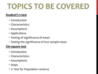
1. TOPICS TO BE COVERED
Student’s t-test
• Introduction
• Characteristics
• Assumptions
• Applications
• Testing of significance of mean
• Testing the significance of two sample mean
Chi-square test
• Introduction
• Characteristics
• Assumptions
• Steps
• x2 Test for Population variance

2. Student’s t-test

3. INTRODUCTION
Student’s t-distributions used to carry out test
of significance for small samples. It is required
for the estimation of samples whenever the
sample size is 30 or less than 30 and standard
deviation of population is not known.

4.  The t-distribution is bell shaped and symmetrical.
 A t-distribution is lower at the mean and higher at the tails.
 It ranges from negative infinity to positive infinity.
 The t-distribution is flatter than normal distribution.
 The variance of the t-distribution is more than one but
approaches one as the degree of freedom and size of sample
increases.
 The statistic of t-distribution depends on degree of freedom.
CHARACTERISTICS

5.  The population from which small samples has been
selected is normal.
 The samples are random.
 The standard deviation of population is unknown.
ASSUMPTIONS

6.  To test the significance of the mean of the random sample,
population variance being unknown.
 To test the significance of the difference between two sample
means (independent samples).
 To test the significance of difference between two sample
means (dependent samples).
 To test the significance of an observed correlation coefficient.
APPLICATIONS

7. TESTING OF SIGNIFICANCE OF
MEAN
 NULL HYPOTHESIS: T-distribution is a continuous distribution
where the value of mean, mode and median is zero or can be
zero.
𝑯𝟎 = 𝑿 = 𝝁
𝑯𝒂 = 𝑿 ≠ 𝝁
 LEVEL OF SIGNIFICANCE: Usually the hypothesis is tested at 5%
or 1% level of significance.

8.  UNBAISED ESTIMATE OF POPULATION: Since the standard deviation of
population is unknown, therefore in place of it, it’s unbiased estimate is
used: (Population of standard deviation)
 CALCULATION OF T-STATISTIC:
𝑿 − 𝝁
𝑺
∗ 𝒏
In place of 𝑆 (if it is unbiased) we use sample standard deviation i.e. ‘S’
Then to calculate the value of T- statistics, we use the following formula:
𝑻 =
𝑿 − 𝝁
𝑺
𝒏 − 𝟏
𝑺 =
𝒅 𝟐
𝒏
𝑺 =
𝒅 𝟐
𝒏 − 𝟏 𝒅 𝟐
= 𝒙 − 𝑿 𝟐

9.  CRITICAL VALUE OF T: Critical value or tabulated value of t is
obtained at a specified level of significance for (n-1) degree of
freedom.
 Decision: If the calculated value of t is more than tabulated value,
it falls in the rejection region and the null hypothesis is rejected
and we can say the difference between mean of sample and mean
of population is significant. On the contrary, if the calculated value
of t is less than tabulated value, we accept the null hypothesis and
we can say the difference between mean of sample and mean of
population is insignificant.

10. PAIRED T - TEST
 The significance of difference between two sample means.
 The difference between means of two samples is significant or
insignificant weather both the samples have been drawn independently
from the same population or not.
To ascertain it the test of significance of difference between two
samples (paired test) shall be worked out through T-test.
To calculate T-statistic, we use following formula:
𝒕 =
𝑿 𝟏 − 𝑿 𝟐
𝑺
𝟏
𝒏 𝟏
+
𝟏
𝒏 𝟐
OR
𝒕 =
𝑿 𝟏 − 𝑿 𝟐
𝑺
∗
𝒏 𝟏 ∗ 𝒏 𝟐
𝒏 𝟏 + 𝒏 𝟐

11. The combined estimate of standard deviation ( 𝑆) is calculated by following
formula:
𝑺 =
𝑿 𝟏 − 𝑿 𝟏
𝟐 + 𝑿 𝟐 − 𝑿 𝟐
𝟐
𝒏 𝟏 − 𝟏 ∗ (𝒏 𝟐 − 𝟏)
OR 𝑺 =
𝒅 𝟏
𝟐
+ 𝒅 𝟐
𝟐
𝒏 𝟏 + 𝒏 𝟐 − 𝟐
But in case where mean values are in fraction then we can use shortcut method
formula i.e.
Deviation must be taken from assumed mean and then combined estimate of
standard deviation. Calculated as follows:
𝑺 =
𝑿 𝟏 − 𝑨 𝟏
𝟐 + 𝑿 𝟐 − 𝑨 𝟐
𝟐 − 𝒏 𝟏( 𝑿 𝟏 − 𝑨 𝟏) 𝟐−𝒏 𝟐( 𝑿 𝟐 − 𝑨 𝟐) 𝟐
𝒏 𝟏 + 𝒏 𝟐 − 𝟐
If variance and direct values are given we can use this formula:
𝑺 =
𝒏 𝟏 𝑺 𝟏
𝟐
+ 𝒏 𝟐 𝑺 𝟐
𝟐
𝒏 𝟏 + 𝒏 𝟐 − 𝟐
Degree of Freedom:
𝒏 𝟏 − 𝟏 ∗ (𝒏 𝟐 − 𝟏)

12. CHI-SQUARE
TEST (X2 TEST)

13. The chi-square test is used to determine if the two attributes
are independent of each other.
It is a measure to evaluate the difference between observed
frequencies and expected frequencies to examine whether
the difference so obtained is due to a chance factor or
sampling factor.
INTRODUCTION

14.  Chi-square test is based on frequencies not on parameters.
 It is a non-parametric test where no parameters regarding the
rigidity of population or populations are required.
 Adaptive property is also found in chi-square test.
 Chi-square test is useful to test the hypothesis about the
independence of attributes.
CHARACTERISTICS

15.  The sample should be selected randomly.
 All-items of sample should be independent of each other.
 The total number of items i.e. N shared reasonably be larger.
It is very difficult to say about largeness but generally the N
should be more than 50.
 The constraints on cell frequencies should be linear.
ASSUMPTIONS

16. STEPS OF CHI-SQUARE
CALCULATION
Step 1 Null Hypothesis
Step 2 Calculation of Expected frequencies
Step 3 Difference between observed and Expected frequencies
Step 4 Square of Column value arrived at Step 3
Step 5 Square divided by the Expected Frequencies

17. X2 TEST FOR POPULATION
VARIANCE
The chi-square test enable us to test whether the
sample has been drawn from normal population in
which the variance is a specified value or not.

18. PROCEDURE
 NULL HYPOTHESIS :
𝑯 𝟎: 𝝈 𝟐 = 𝑺 𝟐
i.e. there is no significant difference between the variance of sample and
population or sample as been drawn from the population in which variance
is a specified value.

19.  TEST STATISTIC FOR POPULATION VARIANCE:
 DEGREE OF FREEDOM: 𝒏 − 𝟏
 DECISION:
The computed value of x2 is compared with the critical value of x2 at a
specific level of significance on the basis of which null hypothesis is
accepted or rejected.
𝒙 𝟐 =
(𝑿 − 𝑿) 𝟐
𝝈 𝟐
OR
𝒏𝑺 𝟐
𝝈 𝟐