Random matrix theory has long been used to study the spectral properties of physical systems, and has led to a rich interplay between probability theory and physics [1]. Historically, random matrices have been used to model physical systems with random fluctuations, or systems whose eigenproblems were too difficult to solve numerically. This talk explores applications of RMT to the physics of disorder in organic semiconductors [2,3]. Revisiting the old problem of Anderson localization [4] has shed new light on the emerging field of free probability theory [5]. I will discuss the implications of free probabilistic ideas for finite-dimensional random matrices [6], as well as some hypotheses about eigenvector locality. Algorithms are available in the RandomMatrices.jl package [7] written for the Julia programming language. [1] M. L. Mehta. Random matrices, 3/e, Academic Press, 2000. [2] J. Chen, E. Hontz, J. Moix, M. Welborn, T. Van Voorhis, A. Suarez, R. Movassagh, and A. Edelman. Error analysis of free probability approximations to the density of states of disordered systems. Phys. Rev. Lett. (2012) 109:36403. [3] M. Welborn, J. Chen, and T. Van Voorhis. Densities of states for disordered systems from free probability. Phys. Rev. B (2013) 88:205113. [4] P. W. Anderson. Absence of diffusion in certain random lattices. Phys. Rev. (1958) 109:1492--1505. [5] D. Voiculescu. Addition of certain non-commuting random variables. J. Functional Anal. (1986) 66:323--346. [6] J. Chen, T. Van Voorhis, and A. Edelman. Partial freeness of random matrices. arXiv:1204.2257 [7] https://github.com/jiahao/RandomMatrices.jl

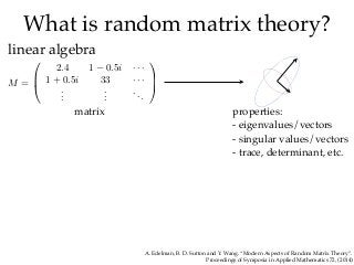
1. What is random matrix theory?
linear algebra
matrix properties:
- eigenvalues/vectors
- singular values/vectors
- trace, determinant, etc.
M =
⎛
⎜
⎝
2.4 1 − 0.5i · · ·
1 + 0.5i 33 · · ·
...
...
...
⎞
⎟
⎠
A. Edelman, B. D. Sutton and Y. Wang. “Modern Aspects of Random Matrix Theory”.
Proceedings of Symposia in Applied Mathematics 72, (2014)

2. What is random matrix theory?
linear algebra
matrix properties:
- eigenvalues/vectors
- singular values/vectors
- trace, determinant, etc.
M =
⎛
⎜
⎝
2.4 1 − 0.5i · · ·
1 + 0.5i 33 · · ·
...
...
...
⎞
⎟
⎠
A. Edelman, B. D. Sutton and Y. Wang. “Modern Aspects of Random Matrix Theory”.
Proceedings of Symposia in Applied Mathematics 72, (2014)
random matrix theory
ensemble of matrices
M =
⎛
⎜
⎝
g g · · ·
g g · · ·
...
...
...
⎞
⎟
⎠
ensemble of matrix properties
Noteb

3. 1. The semicircle law
M =
⎛
⎜
⎝
g g · · ·
g g · · ·
...
...
...
⎞
⎟
⎠
n=500
M=randn(n, n)
M=(M+M’)/√2n
hist(eigvals(M))
E P Wigner, Ann. Math. 62 (1955), 548; 67 (1958), 325
−4 −3 −2 −1 0 1 2 3 4
0
0.05
0.1
0.15
0.2
0.25
0.3
0.35
0.4
0.45
−4 −3 −2 −1 0 1 2 3 4
0
0.05
0.1
0.15
0.2
0.25
0.3
0.35
0.4
0.45
−4 −3 −2 −1 0 1 2 3 4
0
0.05
0.1
0.15
0.2
0.25
0.3
0.35
0.4
0.45
−4 −3 −2 −1 0 1 2 3 4
0
0.05
0.1
0.15
0.2
0.25
0.3
0.35
0.4
0.45
−4 −3 −2 −1 0 1 2 3 4
0
0.05
0.1
0.15
0.2
0.25
0.3
0.35
0.4
0.45
−4 −3 −2 −1 0 1 2 3 4
0
0.05
0.1
0.15
0.2
0.25
0.3
0.35
0.4
0.45
−4 −3 −2 −1 0 1 2 3 4
0
0.05
0.1
0.15
0.2
0.25
0.3
0.35
0.4
0.45
−4 −3 −2 −1 0 1 2 3 4
0
0.05
0.1
0.15
0.2
0.25
0.3
0.35
0.4
0.45
−4 −3 −2 −1 0 1 2 3 4
0
0.05
0.1
0.15
0.2
0.25
0.3
0.35
0.4
0.45
distribution of
eigenvalues
Notebook

4. histogram of level spacings
2. Level spacings: nuclear transitions
M. L. Mehta, “Random Matrices” 3/e (2004), Ch. 1energy levels
level
spacings
uncorrelated eigenvalues
“randomly” correlated
eigenvalues
distribution of eigenvalue gaps
= distribution of nuclear energy levels

5. 0 0.5 1 1.5 2 2.5 3 3.5
0
0.2
0.4
0.6
0.8
1
1.2
bus spacing
P(s)
s
Figure1. BusintervaldistributionP(s) obtainedforcitylinenumberfour. Thefullcurverepresents
the random matrix prediction (4), the markers (+) represent the bus interval data and bars display
the random matrix prediction (4) with 0.8% of the data rejected.
2. Level spacings: bus arrival times
Nextbus.com/MBTA real-time data
12/6/2012 and 12/7/2012
Picture: transitboston.com
bus intervals in Cuernavaca, Mexico
Krbálek and Šeba, J. Phys. A 33 (2000) L229

6. 0 0.5 1 1.5 2 2.5 3 3.5
0
0.2
0.4
0.6
0.8
1
1.2
bus spacing
P(s)
s
Figure1. BusintervaldistributionP(s) obtainedforcitylinenumberfour. Thefullcurverepresents
the random matrix prediction (4), the markers (+) represent the bus interval data and bars display
the random matrix prediction (4) with 0.8% of the data rejected.
2. Level spacings: bus arrival times
bus intervals in Cuernavaca, Mexico
Krbálek and Šeba, J. Phys. A 33 (2000) L229
mean

7. 3. Growth & the Tracy-Widom Law
−5 −4 −3 −2 −1 0 1 2
0
0.05
0.1
0.15
0.2
0.25
0.3
0.35
0.4
0.45
0.5
K A Takeuchi and M Sano J. Stat. Phys. 147 (2012) 853
C A Tracy and H Widom, Phys. Lett. B 305 (1993) 115; Commun.
Math. Phys. 159 (1994), 151; 177 (1996), 727
experimental fluctuations of phase boundary = theoretical fluctuations in Gaussian ensembles
phase interface in a liquid crystal
statistics of fluctuations:
skewness, kurtosis
distribution of largest
eigenvalue
−2.5 −2 −1.5 −1 −0.5 0 0.5 1 1.5 2 2.5
−0.1
0
0.1
0.2
0.3
0.4
M =
⎛
⎜
⎝
g g · · ·
g g · · ·
...
...
...
⎞
⎟
⎠
largest eigenvalue of a random matrix

8. Physical consequences of disorder
❖ Electrical resistance in metals
thermal fluctuations
lattice defects
chemical impurities
❖ Spontaneous magnetization
ergodicity breaking
spontaneous symmetry breaking
❖ Dynamical localization
interference between paths suppresses
transport
Pictures: Wikipedia
ahmedmater.com
UPAA MIC Winners, Sep. 2011

9. Why is the semicircle law true?
E P Wigner, Ann. Math. 62 (1955), 548; 67 (1958), 325
Notebook
Wigner’s original proof:
Compute all moments of the eigenvalue distribution
Recall:
For a matrix M, the nth moment of its spectral density is the
expected trace of Mn. Denote this quantity as <Mn>.

10. Why is the semicircle law true?
E P Wigner, Ann. Math. 62 (1955), 548; 67 (1958), 325
The expected trace of Mn is actually a long sum of expectations

11. Why is the semicircle law true?
E P Wigner, Ann. Math. 62 (1955), 548; 67 (1958), 325
The expected trace of Mn is actually a long sum of expectations

12. Why is the semicircle law true?
E P Wigner, Ann. Math. 62 (1955), 548; 67 (1958), 325
The expected trace of Mn is actually a long sum of expectations
= N-1 paths of weight 1
+ 1 path of weight 1
on average
= N

13. Why is the semicircle law true?
E P Wigner, Ann. Math. 62 (1955), 548; 67 (1958), 325
The only distribution with these moments is the semicircle law
(using Carleman, 1923).
= N-1 paths of weight 1
+ 1 path of weight 1
on average
= N

14. Can we add eigenvalues?
In general, no. One must add eigenvalues vectorially.
eig(A) + eig(B) = eig(A+B) ?
1 + 1 = 2
vector 1
direction = eigenvector of A
magnitude = eigenvalue of A
vector 2
direction = eigenvector of B
magnitude = eigenvalue of Bvector sum
direction = eigenvector of A+B
magnitude = eigenvalue of A+B

15. Special cases of “matrix sums”
eigenvector of A
eigenvalue of A
eigenvector of B
eigenvalue of B
eigenvector of A+B
eigenvalue of A+B
Case 1. A and B commute.
A and B have the same basis, i.e. all their
corresponding eigenvectors are parallel.
Case 2. A and B are in general position.
The bases of A and B are randomly oriented
and have no preferred directions in common.
No deterministic analogue!
The eigenvalue distribution (density of states)
of A + B is the free convolution of the separate
densities of states.
=
A. Nica and R. Speicher, Lectures on the Combinatorics of Free Probability, 2006
JC and A Edelman, arXiv:1204.2257
Generalization to random matrices:
The eigenvalue distribution (density of states)
of A + B is the convolution of the separate
densities of states.
=*

16. Free convolutions
Case 2. A and B are in general position.
The bases of A and B are randomly oriented
and have no preferred directions in common.
The eigenvalue distribution (density of states)
of A + B is the free convolution of the separate
densities of states.
=
D. Voiculescu, Inventiones Mathematicae, 1991, 201-220.
function eigvals_free(A, B)
n = size(A, 1)
Q = qr(randn(n, n))
M = A + Q*B*Q’
eigvals(M)
end
The spectral density of M can be
given by free probability theory

17. Noisy electronic structure
Tight binding Anderson Hamiltonian in 1D
constant coupling
Gaussian disorder
interaction
J
+
random fluctuation of site energies

18. Avoiding diagonalization
In general, exact diagonalization is expensive.
Strategy: split H into pieces with known eigenvalues
then recombine using free convolution. How accurate is it?
−4 −3 −2 −1 0 1 2 3 4
0
0.05
0.1
0.15
0.2
0.25
0.3
0.35
0.4
0.45

19. Results of free convolution
Approximation
Exact
high noise moderate noise low noise
JC et al. Phys. Rev. Lett. 109 (2012),
036403

20. -10
0
10 0.1
1
10
0
0.1
0.2
ρ(x)
x
σ/J
ρ(x)
-10
0
10 0.1
1
10
0
0.1
0.2
ρ(x)
x
σ/J
ρ(x)
2D square 2D honeycomb
-10
0
10 0.1
1
10
0
0.1
0.2
ρ(x)
x
σ/J
ρ(x)
3D cube
-10
0
10 0.1
1
10
0
0.1
0.2
0.3
ρ(x)
x
σ/J
ρ(x)
1D next-nearest neighbors
-10
0
10 0.1
1
10
0
0.1
0.2
ρ(x)
x
σ*/σ
ρ(x)
1D NN with fluctuating interactions
exact
approx.

21. Spectral signature of localization
Spectral compressibility
0 for Wigner statistics (maximally delocalized states)
1 for Poisson statistics (localized states)
measures fine-scale fluctuations in the level density
Can tell something about eigenvectors from the eigenvalues?!
B. L. Altshuler, I. K. Zharekeshev, S. A. Kotochigova, and B. I. Shklovskii, Sov. Phys. JETP 67 (1988) 625.
Relationships between c and localization length of eigenvectors are
conjectured to hold for certain random matrix ensembles
χ(E) = lim
⟨N(E)⟩→∞
d ∆N2
(E)
d ⟨N(E)⟩
∼
∆N2
(E)
⟨N(E)⟩

22. Excitation energy (eV)
RMSlength(normalized)
1.6 1.8 2 2.2 2.4
0.2
0.4
0.6
0.8
Can tell something about eigenvectors from the eigenvalues?!
Spectral signature of localization
spectral compressibility

24. Strategy 1. Model Hamiltonians
atomic coordinates electronic structure
dynamics
observable
disordered system
ensemble-averaged
observable
sampling in
phase space
...
ensemble of
model
Hamiltonians

25. Outline
❖ Introduction: organic solar cells
Bulk heterojunctions
Disorder matters!
Computing
❖ Disordered excitons ab initio
The sampling challenge
Exciton band structures
❖ Models for disordered excitons
Random matrix theory
Quantum mechanics without wavefunctions
±
+
Excitation energy (eV)
Localizationlength(normalized)
1.4 1.6 1.8 2 2.2 2.4
0
0.2
0.4
0.6
0.8

26. A standard protocol of
computational chemistry
crystal atomic coordinates
electronic structure
dynamics
observable

27. A standard protocol of
computational chemistry
crystal atomic coordinates
electronic structure
dynamics
observable
?X
disordered system

28. disordered system
observable
?
Modeling disorder: explicit sampling

29. Modeling disorder: explicit sampling
disordered system
observable
sampling in
phase space
...
atomic coordinates electronic structure
dynamics
observable
ensemble averaging

30. Q-Chem input
generation
Infrastructure for large-scale
quantum chemical simulations
HDF5
Database
Q-Chem output file parsing
Q-Chem
QM/MM
Grid
Engine
CHARMM
error handling
convergence failures
system failures
...
job dispatcher
queue monitor
error handling for
cluster-wide failures
post-analysis
scripts
sampling electronic structure observables

31. thermalizedperfect crystal
Step 1. Sample thermalized states using molecular dynamics
NVT dynamics of 8x8x8 supercell in CHARMM

33. Cost: ~4 CPU-hours
Step 2. Calculate absorption frequencies (energies) of each
molecule using ab initio electronic structure theory
TD-PBE0/6-31G* with electrostatic embedding in Q-Chem + 0.2 eV shift
*L Edwards and M. Gouterman, J. Mol. Spect. 33 (1970), 292
Qx
Qy
B

34. Step 3. Collect statistics to recover averaged spectra
100 snapshots x 128 molecules, ~6 CPU-years
Absorption spectrum (gas)
1.2 1.4 1.6 1.8 2 2.2
(condensed)
Energy (eV)
Qx
Qy
Qx Qy
tail states?

35. • Normalized root mean square spread
of the exciton wavefunction
• Localization determines nature of transport
Localization of states
1
N 1
l =
1
Lmax
ψ |r|
2
ψ − ⟨ψ |r| ψ⟩
2
incoherent
diffusive
coherent
ballistic

36. Localization of states
Excitation energy (eV)
RMSlength(normalized)
1.6 1.8 2 2.2 2.4
0.2
0.4
0.6
0.8

37. Localization of states
Excitation energy (eV)
RMSlength(normalized)
1.6 1.8 2 2.2 2.4
0.2
0.4
0.6
0.8
delocalized

38. Localization of states
Excitation energy (eV)
RMSlength(normalized)
1.6 1.8 2 2.2 2.4
0.2
0.4
0.6
0.8
0 50 100 20
40
60
60
80
100
120
140
160
180
sample 61, state 5, energy = 2.126573
- delocalized along
herringbone axis only
- antiferromagnetic order
in transition dipoles

39. Localization of states
Excitation energy (eV)
RMSlength(normalized)
1.6 1.8 2 2.2 2.4
0.2
0.4
0.6
0.8
- mostly delocalized along
herringbone axis
- polaron-like
- antiferromagnetic order
in transition dipoles

40. Localization of states
Excitation energy (eV)
RMSlength(normalized)
1.6 1.8 2 2.2 2.4
0.2
0.4
0.6
0.8
0
50
100
20
40
60
60
80
100
120
140
160
180
sample 1, state 51, energy = 1.715239
- mostly delocalized along
herringbone axis
- polaron-like
- ferromagnetic order
in transition dipoles

41. Excitation energy (eV)
RMSlength(normalized)
1.6 1.8 2 2.2 2.4
0.2
0.4
0.6
0.8
Asymmetry from neighbor shells
Excitation energy (eV)
RMSlength(normalized)
1.6 1.8 2 2.2 2.4
0.2
0.4
0.6
0.8
1 2 all
number of
neighbor
shells

42. Neighbor shells in crystal
Excitation energy (eV)
RMSlength(normalized)
1.7 1.75 1.8 1.85 1.9
0.6
0.7
0.8
0.9
1
Excitation energy (eV)
RMSlength(normalized)
1.5 1.6 1.7 1.8 1.9 2
0.8
0.85
0.9
0.95
1
Excitation energy (eV)
RMSlength(normalized)
1.5 1.6 1.7 1.8 1.9 2
0.85
0.9
0.95
1
Excitation energy (eV)
RMSlength(normalized)
1.4 1.6 1.8
0.7
0.75
0.8
0.85
0.9
0.95
1
1 2 3 all
number of
neighbor
shells

43. Summary
Excitons in H2Pc come in
three distinct flavors
high energy:
localized in 2D, delocalized
along herringbone axis
• medium energy:
delocalized
• low energy:
dressed states localized
predominantly in 2D
Asymmetric density of states
is a nonlocal effect
J.C. et al., Phys. Rev. Lett. 2012
Excitation energy (eV)
Localizationlength(normalized)
1.4 1.6 1.8 2 2.2 2.4
0
0.2
0.4
0.6
0.8

44. Modeling disorder
disordered system
observable
sampling in
phase space
...
atomic coordinates electronic structure
dynamics
observable
ensemble averaging

45. Modeling disorder
disordered system
observable
sampling in
phase space
...
atomic coordinates electronic structure
dynamics
observable
ensemble averaging
4 CPU-hours
Absorption spectrum (gas)
1.2 1.4 1.6 1.8 2 2.2
(condensed)
Energy (eV)
6 CPU-years
1 “CPU-PhD”

46. Modeling disorder
atomic coordinates electronic structure
dynamics
observable
disordered system
ensemble-averaged
observable
sampling in
phase space
random matrix theory?
...
spatial disorder
spectral disorder

47. Summary
•Free probability allows us to construct accurate
approximations to analytic model Hamiltonians
•An error analysis of this phenomenon is known
•Statistics of eigenvalues may be able to tell us
information about experimental observations
J.C. et al., Phys. Rev. Lett. 2012