9990611130 Find & Book Russian Call Girls In Vijay Nagar
DOMV No 8 MDOF LINEAR SYSTEMS - RAYLEIGH'S METHOD - FREE VIBRATION.pdf
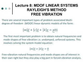
1. Lecture 8: MDOF LINEAR SYSTEMS
RAYLEIGH'S METHOD
FREE VIBRATION
𝑚𝑚 ̈
𝑧𝑧 + 𝑐𝑐 ̇
𝑧𝑧 + 𝑘𝑘 𝑧𝑧 = 𝑝𝑝(t)
There are several important types of problem associated Multi-
degree-of-freedom (MDOF) linear dynamic models of the form:
The first most important problem is to obtain natural frequencies and
mode shapes of free vibration i.e. undamped, unforced systems. This
involves solving the system model equation:
𝑚𝑚 ̈
𝑧𝑧 + 𝑘𝑘 𝑧𝑧 = 0
Free-vibration natural frequencies and mode shapes are of interest in
their own right but they also play a big part in forced vibration analysis.
2. Free Vibration
Given the importance of natural frequencies, historically,
many approximate methods were developed to obtain
free-vibration natural frequencies. Most of these methods
pre-date digital computers and are therefore largely
obsolete. One method however is still important today,
namely Rayleigh’s method.
In this module we will examine:
1/ Free-vibration natural frequencies and mode shapes
2/ Forced vibration analysis for systems with proportional damping.
3. Rayleigh’s method to obtain approximate
natural frequencies
Rayleigh’s methods is a very powerful approximate method to
obtain natural frequencies of both discrete and continuous
systems. It also forms the basis of the Rayleigh-Ritz method which
is important in several areas and widely used in analysis (but we
will not study it in this module).
Rayleigh’s principle
Rayleigh’s method is based on Rayleigh’s Principle. A corollary of
Rayleigh’s Principle states that: “The frequency of vibration of a
conservative system vibrating about an equilibrium position has a
‘stationary value’ in the neighbourhood of a natural mode. This
stationary value is in fact a minimum value in the neighbourhood of
the ‘fundamental’ natural frequency”.
4. Rayleigh’s method to obtain approximate
natural frequencies
So the natural frequency predicted using Rayleigh’s method is at
a ‘turning point’ (in some sense) when a correct vibration mode
shape is used.
One way to use this principle is to consider the kinetic energy T
and potential energy V for some vibration frequency 𝜔𝜔. The
principle then states that
𝑑𝑑
𝑑𝑑𝑑𝑑
𝑇𝑇 + 𝑉𝑉 = 0 (i.e. a ‘turning point’
condition). This condition ultimately gives an (approximate)
equation for the natural frequency 𝜔𝜔 in terms of an assumed
vibration shape.
An alternative route to the same equation is to equate the
maximum potential energy Vmax to the max kinetic energy Tmax.
6. Rayleigh’s method
Max potential energy Vmax = Max kinetic energy Tmax
We saw earlier the expressions for the kinetic and
potential energy of a discrete MDOF system i.e.:
𝑇𝑇 =
1
2
̇
𝑧𝑧𝑇𝑇 𝑚𝑚 ̇
𝑧𝑧
and
𝑉𝑉 =
1
2
𝑧𝑧𝑇𝑇
𝑘𝑘 𝑧𝑧
7. Rayleigh’s method
If we assume that the dynamic system is vibrating harmonically
at frequency 𝜔𝜔 such that:
𝑧𝑧 𝑡𝑡 = ̂
𝑧𝑧𝑒𝑒𝑗𝑗𝑗𝑗𝑗𝑗
where ̂
𝑧𝑧 is an assumed shape of displacement, then:
𝑇𝑇 =
1
2
𝜔𝜔2 ̂
𝑧𝑧𝑇𝑇 𝑚𝑚 ̂
𝑧𝑧𝑒𝑒2𝑗𝑗𝑗𝑗𝑗𝑗
giving:
𝑇𝑇𝑚𝑚𝑚𝑚𝑚𝑚 = +
𝜔𝜔2
2
̂
𝑧𝑧𝑇𝑇 𝑚𝑚 ̂
𝑧𝑧
And similarly:
𝑉𝑉
𝑚𝑚𝑚𝑚𝑚𝑚 =
1
2
̂
𝑧𝑧𝑇𝑇
𝑘𝑘 ̂
𝑧𝑧
8. Rayleigh’s method
By equating maximum kinetic energy to the potential energy i.e.:
𝑇𝑇𝑚𝑚𝑚𝑚𝑚𝑚 = 𝑉𝑉
𝑚𝑚𝑚𝑚𝑚𝑚
we get:
𝜔𝜔2
2
̂
𝑧𝑧𝑇𝑇 𝑚𝑚 ̂
𝑧𝑧 ≅
1
2
̂
𝑧𝑧𝑇𝑇 𝑘𝑘 ̂
𝑧𝑧
or
𝜔𝜔2 =
̂
𝑧𝑧𝑇𝑇
𝑘𝑘 ̂
𝑧𝑧
̂
𝑧𝑧𝑇𝑇 𝑚𝑚 ̂
𝑧𝑧
This is known as Rayleigh’s Quotient for a discrete system. If ̂
𝑧𝑧 is an eigenvector,
𝜔𝜔 is exact. For example the jth natural frequency can be approximated by
𝜔𝜔𝑗𝑗
2
≅
̂
𝑧𝑧𝑗𝑗
𝑇𝑇
𝑘𝑘 ̂
𝑧𝑧𝑗𝑗
̂
𝑧𝑧𝑗𝑗
𝑇𝑇
𝑚𝑚 ̂
𝑧𝑧𝑗𝑗
where ̂
𝑧𝑧𝑗𝑗 is an assumed mode shape of the jth mode.
9. Rayleigh’s method
• For a SDOF system, Rayleigh's Quotient gives the result:
𝜔𝜔2 =
𝑘𝑘
𝑚𝑚
(which is exact).
• Rayleigh’s Quotient gives an upper bound estimate of 𝜔𝜔1 (i.e. the
lowest natural frequency, known as the ‘fundamental’). For any
assumed mode shape, the true natural frequency of the
fundamental mode is therefore always less than estimated, i.e.
the true fundamental frequency 𝜔𝜔1
2
≤
̂
𝑧𝑧𝑗𝑗
𝑇𝑇
𝑘𝑘 ̂
𝑧𝑧𝑗𝑗
̂
𝑧𝑧𝑗𝑗
𝑇𝑇
𝑚𝑚 ̂
𝑧𝑧𝑗𝑗
.
10. Rayleigh’s method
An Example
For the lumped mass system shown the discrete model is:
𝑚𝑚 0
0 𝑚𝑚
̈
𝑧𝑧1
̈
𝑧𝑧2
+
2𝑘𝑘 − 𝑘𝑘
−𝑘𝑘 2𝑘𝑘
𝑧𝑧1
𝑧𝑧2
=
0
0
We have not studied them yet, but this system has eigenvalues
(exact natural frequencies (squared)):
𝜔𝜔1
2
=
𝑘𝑘
𝑚𝑚
; and 𝜔𝜔2
2
=
3𝑘𝑘
𝑚𝑚
and eigenvectors are:
̂
𝑧𝑧(1) =
1
1
and ̂
𝑧𝑧(2) =
1
−1
.
We are actually trying to estimate 𝜔𝜔1
11. Rayleigh’s method
Note: If we put the true mode shapes into Rayleigh's Quotient we will
obtain the exact natural frequencies i.e.
1 1
2𝑘𝑘 − 𝑘𝑘
−𝑘𝑘 2𝑘𝑘
1
1
= 2𝑘𝑘 ; 1 1
𝑚𝑚 0
0 𝑚𝑚
1
1
= 2𝑚𝑚
𝜔𝜔𝑗𝑗
2
≅
̂
𝑧𝑧𝑗𝑗
𝑇𝑇
𝑘𝑘 ̂
𝑧𝑧𝑗𝑗
̂
𝑧𝑧𝑗𝑗
𝑇𝑇
𝑚𝑚 ̂
𝑧𝑧𝑗𝑗
∴ 𝜔𝜔1
2
=
2𝑘𝑘
2𝑚𝑚
=
𝑘𝑘
𝑚𝑚
(which is exact); and if we use
1
−1
𝜔𝜔2
2
=
3𝑘𝑘
𝑚𝑚
(also exact )
12. Rayleigh’s method
Suppose however the guess of the 1st mode shape were ̂
𝑧𝑧(1) =
1
0.5
(not
1
1
) then:
𝜔𝜔1
2
≅
̂
𝑧𝑧𝑇𝑇
𝑘𝑘 ̂
𝑧𝑧
̂
𝑧𝑧𝑇𝑇 𝑚𝑚 ̂
𝑧𝑧
=
1 0.5
2𝑘𝑘 − 𝑘𝑘
−𝑘𝑘 2𝑘𝑘
1
0.5
1 0.5
𝑚𝑚 0
0 𝑚𝑚
1
0.5
=
6
5
𝑘𝑘
𝑚𝑚
>
𝑘𝑘
𝑚𝑚
𝜔𝜔1 = 1.095
𝑘𝑘
𝑚𝑚
i.e. 10% above the true value 𝜔𝜔1 for a large error in 𝑧𝑧(1). If the guess were ̂
𝑧𝑧 1 =
1
0.9
then:
𝜔𝜔1
2
≅
1 0.9
2𝑘𝑘 − 𝑘𝑘
−𝑘𝑘 2𝑘𝑘
1
0.9
1 0.9
𝑚𝑚 0
0 𝑚𝑚
1
0.9
=
1.82𝑘𝑘
1.81𝑚𝑚
= 1.0055
𝑘𝑘
𝑚𝑚
i.e. a 0.3% error in 𝜔𝜔1. Similar accuracy is obtained for estimates of 𝜔𝜔2 but we cannot
say whether the estimates of 𝜔𝜔2 will be above or below the true 𝜔𝜔2).
13. FREE VIBRATION OF LINEAR MDOF
SYSTEMS
This section is concerned with exact calculation of natural
frequencies and mode shapes associated with:
𝑚𝑚 ̈
𝑍𝑍 + 𝑘𝑘 𝑍𝑍 = 𝑂𝑂
which represents free motion associated with an undamped system.
Free vibration characteristics are needed for: i) qualitative use in
assessing potentially problematic frequencies where resonance
could occur in lightly damped systems, and ii) of equal importance,
to obtain normal modes which can be used to solve MDOF systems
with forcing and proportional damping. Here the focus will be on
systems with a symmetric matrices for [m] and [k].
14. FREE VIBRATION OF LINEAR MDOF
SYSTEMS
Mathematically the problem to solve requires solution of the
eigenvalues and eigenvectors of a square (but not
necessarily symmetric) matrix. For a conservative system
given by:
both the eigenvalues and eigenvectors are real. So the focus
will be the interpretation of the eigenvalues and vectors. The
derivation of some important orthogonality properties which
the normal modes satisfy will be given in the next
presentation.
𝑚𝑚 ̈
𝑍𝑍 + 𝑘𝑘 𝑍𝑍 = 𝑂𝑂
15. FREE VIBRATION OF LINEAR MDOF
SYSTEMS
Eigenvalues and Eigen Vectors of Conservative Systems
To obtain the solution for model 𝑚𝑚 ̈
𝑍𝑍 + 𝑘𝑘 𝑍𝑍 = O we assume
the solution is harmonic of complex amplitude (i.e. sinusoidal or
co-sinusoidal) which allows phase shift between input and
output to be easily accounted for. Therefore assume:
𝑍𝑍 𝑡𝑡 = ̂
𝑍𝑍𝑒𝑒𝑖𝑖𝑖𝑖𝑖𝑖
where ̂
𝑍𝑍 is a constant vector with complex components, which
on substitution into the model gives:
−𝜔𝜔2
𝑚𝑚 ̂
𝑍𝑍 + 𝑘𝑘 ̂
𝑍𝑍 𝑒𝑒𝑖𝑖𝑖𝑖𝑖𝑖
= 0
but since:
𝑒𝑒𝑖𝑖𝑖𝑖𝑖𝑖 ≠ 0
gives:
−𝜔𝜔2 𝑚𝑚 ̂
𝑍𝑍 + 𝑘𝑘 ̂
𝑍𝑍 = 0
16. FREE VIBRATION OF LINEAR MDOF
SYSTEMS
Now pre-multiply −𝜔𝜔2 𝑚𝑚 ̂
𝑍𝑍 + 𝑘𝑘 ̂
𝑍𝑍 = 0 by 𝑚𝑚 −1 (assuming it exists), we obtain:
𝐸𝐸 − 𝜔𝜔2
𝐼𝐼 ̂
𝑍𝑍 = 0
where 𝐸𝐸 = 𝑚𝑚 −1
𝑘𝑘 is known as the Stiffness Form of the Dynamic Matrix.
This is a standard eigenvalue problem in which (ascending order) eigenvalues
𝜔𝜔2 of the matrix E need to be found. Corresponding vectors ̂
𝑍𝑍 which satisfy
the above equation at each of the eigenvalues also need to be found. The
eigenvalues and eigenvectors are interpreted as Natural Frequencies and
Modes Shapes of vibration respectively for free undamped vibration. These
eigenvectors are called Normal Modes.
Note: the standard eigenvalue problem associated with a square matrix A is
usually written in the form 𝐴𝐴 − λ𝐼𝐼 𝑥𝑥 = 0.
17. FREE VIBRATION OF LINEAR MDOF
SYSTEMS
Now the solution process to obtain the eigenvalues and eigenvectors is
only possible if:
𝐸𝐸 − 𝜔𝜔2
𝐼𝐼 = 0
i.e. a determinantal equation which leads to the frequency equation (i.e. a
polynomial in 𝜔𝜔2) the roots of which are the eigenvalues ( 𝜔𝜔1
2
, 𝜔𝜔2
2
, … , 𝜔𝜔𝑁𝑁
2
.
There should be N roots. Now 𝜔𝜔1 is called the first mode frequency (or the
fundamental frequency), 𝜔𝜔2 is the 2nd mode frequency, and so on. If, for
each eigenvalue, we substitute back into: 𝐸𝐸 − 𝜔𝜔𝑖𝑖
2
Ι ̂
𝑍𝑍 = 0 then from this
equation, we can solve for an eigenvector which is a relative measure of
how the displacements are related, when the system is vibrating in the ith
mode, with frequency 𝜔𝜔𝑖𝑖. The eigenvector only tells us the relative shape of
the free vibration – the amplitudes can be anything. Often, the amplitude of
displacement for the first component is conveniently set = 1; the vector
may also be normalised to magnitude = 1 (as explained shortly).
18. FREE VIBRATION OF LINEAR MDOF
SYSTEMS
Example: Computing the Natural Frequencies and Mode shapes:
A 3-DOF system (taken from Newland p125, involving simple hand calculation).
The system is a 3 x 3 system lumped mass model of equal mass m and equal
stiffness k as shown in the figure. The model is:
𝑚𝑚 ̈
𝑧𝑧 + 𝑐𝑐 ̇
𝑧𝑧 + 𝜅𝜅 𝑧𝑧 = 0
which has mass, stiffness, and damping matrices as follows:
𝑚𝑚 =
𝑚𝑚 0 0
0 𝑚𝑚 0
0 0 𝑚𝑚
𝑘𝑘 =
2𝑘𝑘 −𝑘𝑘 0
−𝑘𝑘 2𝑘𝑘 −𝑘𝑘
0 −𝑘𝑘 2𝑘𝑘
𝑐𝑐 = [0]
Here we choose value 𝑚𝑚 = 1.0 kg and stiffness 𝑘𝑘 = 1.0 N/m for this system
19. FREE VIBRATION OF LINEAR MDOF
SYSTEMS
𝑚𝑚−1 =
1/𝑚𝑚 0 0
0 1/𝑚𝑚 0
0 0 1/𝑚𝑚
; 𝑚𝑚−1𝜅𝜅 =
2 −1 0
−1 2 −1
0 −1 2
= 𝐸𝐸
To obtain the eigenvalues, we solve: 𝐸𝐸 − 𝜔𝜔2Ι = 0 which leads to finding the roots
of a cubic polynomial in 𝜔𝜔2. The roots are:
𝜔𝜔1
2
= 0.5858 𝜔𝜔1 = 0.7654 rad/sec
𝜔𝜔2
2
= 2.0000 𝜔𝜔2 = 1.4142 rad/sec
𝜔𝜔3
2
= 3.4142 𝜔𝜔3 = 1.8478 rad/sec
And for each 𝜔𝜔𝑖𝑖 we can obtain eigenvectors by setting the first component in the
vector 𝑍𝑍1 = 1 and solving the remaining linear equations. Following this procedure
gives the eigenvectors:
𝑍𝑍(1) =
1.0
2
1.0
𝑍𝑍(2) =
1.0
0.0
−1.0
𝑍𝑍(3) =
1.0
− 2
1.0
𝜔𝜔1 𝜔𝜔2 𝜔𝜔3
So the 1st element is arbitrarily normalised to 1.
20. FREE VIBRATION OF LINEAR MDOF
SYSTEMS
The eigenvectors show the relative
amplitudes when the structure is vibrating
only at that corresponding natural frequency.
We can show these eigenvectors graphically in
the form of mode shapes, which give relative
vibrations for each of the modes.
21. FREE VIBRATION OF LINEAR MDOF
SYSTEMS
The mode shapes:
1
.
0
1
.
0
Mode 1
1
.
0
1
.
0
Mode 2
at 𝜔𝜔1
at 𝜔𝜔2
at 𝜔𝜔3
1
.
0
Mode 3
1
.
0
22. FREE VIBRATION OF LINEAR MDOF
SYSTEMS
Normalisation of Eigenvectors
It is often convenient to rescale the eigenvectors to different lengths. Sometimes
this might be (as in FE code) to make the largest amplitude 1 (as we have already
done). Another procedure is to make the eigenvectors have length 1 (as in Matlab)
i.e. to scale the eigenvectors as follows:
𝑢𝑢(1) =
𝑍𝑍(1)
𝑍𝑍 1
, 𝑢𝑢(2) =
𝑍𝑍(2)
𝑍𝑍(2)
, 𝑢𝑢(3) =
𝑍𝑍(3)
𝑍𝑍(3)
, … , 𝑢𝑢(𝑁𝑁) =
𝑍𝑍(𝑁𝑁)
𝑍𝑍(𝑁𝑁)
For the previous 3 x 3 system example, the unit-length normalised eigenvectors
are:
𝑢𝑢(1) =
𝑍𝑍(1)
𝑍𝑍 1
=
1
12+ 2
2
+12
�
1
2
1.0
2
1.0
=
1
2
1.0
2
1.0
=
⁄
1.0
2
�
1
2
⁄
1
2
𝑖𝑖. 𝑒𝑒. 𝑢𝑢(1) = 1
24. FREE VIBRATION OF LINEAR MDOF
SYSTEMS
The Modal Matrix
It is common to arrange the Normalised eigenvectors into a special matrix as
follows:
U = 𝑢𝑢(1), 𝑢𝑢 2 , … , 𝑢𝑢(𝑁𝑁)
For the 3 x 3 example, the modal matrix [U] is:
U =
⁄
1
2 �
1
2
⁄
1
2
�
1
2
0 �
−1.0
2
⁄
1
2 �
−1
2
⁄
1
2
The modal matrix for the previous example.
The modal matrix [U] is an important matrix which allows a system of
equations, under certain conditions, to be diagonalised. We will examine this
feature in the next lecture.