This document summarizes the key findings from a study examining terrestrial sediment dynamics in a small tropical reef embayment. The study investigated: 1) Where sediment is coming from using measurements of sediment yield from different sources; 2) How water circulates over the reef using both fixed and drifting sensors under different wind/wave conditions; and 3) Where sediment is accumulating spatially and temporally using sediment traps and pods. Key findings include that the quarry was a major sediment source, northern areas of the reef experienced higher accumulation, and wave energy influences circulation and redistributes carbonate sediment. The interplay between watershed sediment input, hydrodynamics, and accumulation patterns was examined.
Forensic Biology & Its biological significance.pdf
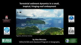
Messina dissertation defense-4_27_16
1. Terrestrial sediment dynamics in a small,
tropical, fringing-reef embayment
by Alex Messina
SDSU/UCSB Joint-Doctoral Program in Geography
photo: Messina
N
Pago Pago
Harbor
Pacific
Ocean
South
ReefNorth
Reef
Stream
Outlet
Faga’alu, American Samoa
2. Motivation and Research questions
Chapter 1: Where is sediment coming from?
and What to do about it?
Chapter 2: How does water circulate over the reef?
Chapter 3: Where is sediment accumulating on the reef?
Sediment accumulation in Faga’alu, Jan 2012
video: Messina
Sediment harming coral in Faga’alu
1. Watershed inputs 2. Hydrodynamics 3. Sediment Accumulation
RIDGE to REEF
3. Chapter 1: Where is sediment coming from?
Sediment from Natural Sources and Human Sources
Human sources:
• Quarry
• Storm drains
• Roads
Natural sediment from forest
QuarryRoad runoff Storm drains
4. Subwatersheds isolate sediment sources:
Natural, quarry, village
2 PT’s (Pressure Transducers)
2 Turbidimeters
1 Autosampler
1 Grad student
Sediment yield measured at
three locations using:
QUARRY
10km
5. Measurements:
• Water discharge (Q) (L/sec)
• Suspended Sediment Concentration (SSC) (mg/L)
Depth with pressure
transducer (PT)
Flow measurements relate
depth to water discharge
(Q, volume/time)
Depth
SSYEV = Q x SSC
1. Measure SSC in water
samples collected by
Autosampler and grab
2. Model SSC from
Turbidity data
Autosampler
Retrieving
samples
Turbidimeter in stream
Grad student
6. Measuring sediment and discharge during storms
Timelapse videos!
Filtering and weighing sediment in laboratory
Auto-sampler
Measuring Q with flow meter
7. Detecting changes in fluvial sediment
Q-SSC problematic due to scatter
1. Discharge-Concentration relationship
2. Changes in annual yields
3. Event-wise analysis
UPSTREAM DOWNSTREAM
CONCENTRATION
DISCHARGE (Q)
FOREST QUARRY VILLAGE
8. Detecting changes in fluvial sediment
Sequential downstream sources are confused
Q-SSC problematic due to scatter
1. Discharge-Concentration relationship
2. Changes in annual yields
3. Event-wise analysis
UPSTREAM DOWNSTREAM
CONCENTRATION
DISCHARGE (Q)
FOREST QUARRY VILLAGE
FOREST QUARRY VILLAGE FOREST QUARRY VILLAGE
Non-storm
Storm
9. Continuous Turbidity
to…
Continuous SSC
Q
(from depth and rating curve)
Integrated over storm
to get total
SSY = Q x SSC
KEY METRIC:
Total SSY from storm event
KEY METRIC:
Total SSY from storm event
TimeStorm
Start
Storm
End
Storm Event
10. SSYEV vs. “Storm Metrics” (precipitation and discharge)
How to compare sediment yield from different sources and events? (1)SSYEV(tons/km2)
Maximum event discharge (Q) (m3/sec/km2)
Example of a “Storm Event”
Maximum Event Q
Total SSYEV
102
101
100
10-1
10-2
10-3
142 Storm Events measured
11. • Compare total and % contributions from sources
• KEY METRIC: Disturbance Ratio (DR):
DR = SSY / SSYFOREST
DR = 1 is no disturbance
How to compare sediment yield from different sources and events? (2)
SSYEV can be used to make a budget of sources
Results from 8 storms
Precip SSYEV (tons)
mm Upper Lower_Quarry Lower_Village Total
Min 12 0.06 0.08 0.3 0.7
Max 86 9.6 8.2 5.3 23.1
Total 299 13.4 16.4 16.0 45.7
% 29 36 35 100
% Area 50 16 34 100
DR 1.0 4.1 1.8 1.7
From 42 storms (UPPER and LOWER only):
• Human-disturbed subwatershed contributed
~87% of SSYEV to the Bay
• Human-disturbed areas have increased SSY
~3.9x above natural yields to the Bay
12. How to compare sediment yield from different sources and events? (2)
SSYEV can be used to make a budget of sources
Results from 8 storms
Precip SSYEV (tons)
mm Upper Lower_Quarry Lower_Village Total
Min 12 0.06 0.08 0.3 0.7
Max 86 9.6 8.2 5.3 23.1
Total 299 13.4 16.4 16.0 45.7
% 29 36 35 100
% Area 50 16 34 100
DR 1.0 4.1 1.8 1.7
SSY from forested and disturbed areas
Upper Lower_Quarry Lower_Village Total
Area disturbed (%) 0.4 6.5 11.7 5.2
Forested areas (tons) 13.3 3.7 7.8 25.0
Disturbed areas (tons) 0.1 12.7 8.2 20.7
% from disturbed areas 1 77 51 45
DR for disturbed areas 3 49 8 15
• Quarry makes up small area but high SSYEV
• High DR at quarry due to constant disturbance
• Compare total and % contributions from sources
• KEY METRIC: Disturbance Ratio (DR):
DR = SSY / SSYFOREST
DR = 1 is no disturbance
From 42 storms (UPPER and LOWER only):
• Human-disturbed subwatershed contributed
~87% of SSYEV to the Bay
• Human-disturbed areas have increased SSY
~3.9x above natural yields to the Bay
13. Conclusions from Chapter 1:
Where is anthropogenic sediment coming from?
Quarry!
• Quarry covered ~1% of watershed,
but contributed ~36% of SSYEV
• Mitigate sediment discharge from quarry
Methodological contributions:
-Automated storm identification
-Quantify change with event-wise SSY
-Disturbance Ratio
Messina, A., Biggs, T. (2016) “Contributions of human activities to
suspended sediment yield during storm events from a small, steep,
tropical watershed.” Journal of Hydrology, in press
Retention ponds installed Oct 2014
14. Chapter Two: How is water circulating over the reef?
Water circulation controls
sediment dynamics
Energetic hydrodynamic forcing
compared with other reefs:
-Variable winds
-Variable waves
-> High spatial variability in
current velocity and direction
How do currents vary spatially over the reef?
How do currents vary under calm conditions, high winds, and high waves?
WIND/WAVES
15. Chapter Two: How is water circulating over the reef?
Water circulation controls
sediment dynamics
Energetic hydrodynamic forcing
compared with other reefs:
-Variable winds
-Variable waves
-> High spatial variability in
current velocity and direction
How do currents vary spatially over the reef?
How do currents vary under calm conditions, high winds, and high waves?
WIND/WAVES
Exposed to big waves!
16. Wave height recorder
Building drifters
3 acoustic current profilers
5 GPS-recording drifters Deployed via paddleboard
EULERIANLAGRANGIAN
METHODS
Two ways to observe flow:
• Eulerian: flow past fixed point
• Lagrangian: follow water parcel
17. Chapter Two: How is water circulating over the reef?
• Lagrangian = spatial coverage
Lagrangian drifters
GPS-tracked drifters, to determine spatial
patterns related to wind and wave forcing
18. Chapter Two: How is water circulating over the reef?
• Eulerian = temporal coverage
Eulerian current meters
Current meters at fixed points to
determine temporal patterns related to
wind and wave forcing
19. Unprecedented spatial coverage:
30 deployments of 5 drifters
Wide range of forcing conditions -> “end members”
Gridded drifter observations: 100m x 100m
Divided into three periods,
isolating forcing conditions:
-Tide (Calm)
-Strong onshore winds
-Large waves
100 m
100m
20. TIDES (CALM) STRONG WINDS LARGE WAVES
Spatial patterns:
1. Faster speeds, consistent directions
over southern reef (crest)
2. Slower flow, variable direction over
northern reef and channel
Forcing patterns:
1. Tides (calm): Slow speeds, variable directions
2. Strong Winds: Slow speeds, toward stream outlet
3. Large Waves: Fastest speeds, most uniform directions;
clockwise flushing pattern
DRIFTERS: Mean flow speed and direction
Slow, variable direction Slow, onshore direction Fast, clockwise circulation
21. TIDES (CALM) STRONG WINDS LARGE WAVES
Spatial/Forcing patterns:
•Similar to Drifters, but no spatial
variation over the reef, clockwise pattern
•Contextualize drifter measurements, and
show flow decreases with tide stage
Comparing Eulerian/Lagrangian:
1. Speeds faster for drifters (50-650%):
• Point – Area
• Surface – Water column
• Stokes’ drift
• Sampling/Analytical error
2. Implications
ADCPs: Mean flow speed and direction
Fastest, esp. on southern reefSlow, less variable directionsSlowest, most variable directions
22. Water residence time
Spatial patterns
• Lowest over southern reef (crest)
• Highest over northern reef and near stream outlet
Forcing patterns
• Lowest during large waves
• Highest during calm and strong onshore winds
Implications:
• Stream discharge deflected over northern reef
• Potential for sediment impacts highest over
northern reef, under calm or onshore wind
23. Conclusions from Chapter 2:
How is water circulating over the reef?
• Wave-breaking on southern reef crest strong control on circulation
• Highly heterogeneous currents over short spatial scales
• Stream discharge likely deflected over northern reef and channel
• Lagrangian velocities were faster than Eulerian; can overestimate flow
Methodological contributions:
-Combined Lagrangian/Eulerian approach
-Spatial coverage of drifters over reef flat
-Spatially distributed residence time
-End member forcing
Messina, A., Storlazzi, C., Cheriton, O., Biggs, T. (in review) “Eulerian and Lagrangian measurements of water flow
and residence time in a fringing reef flat-lined embayment: Faga’alu Bay, American Samoa.”
Future work: real-time tracking
24. Chapter 3: WHERE is sediment accumulating?
and WHEN?
What processes control sediment accumulation,
in space and time?
gross and net?
How sediment input and hydrodynamics interact?
Monthly? Seasonal?
Are accumulation rates above harmful levels?
High waves > Low water residence time > prevent deposition & remove deposited sediment
High SSY from watershed
and/or
Low wave-driven circulation
Hypotheses
High sediment accumulation when:
25. Sampling
Gross and Net accumulation
-10 quasi-monthly, for 1 year
- gross -> in TRAPS
- net -> on PODS
“sediment trap” “sediment pod”
Methods:
Sediment Collection & Analysis
Analysis
Grain size and Composition
-fine/coarse fractions separated
-rinsed of salts
-analyzed for composition:
0rganic, Carbonate, Terrigenous
Sieving/Filtering apparatus
Organisms/Gravel removedSediment collection on SCUBA Rinse and Oven-dry
26. Interaction of Waves and SSY
High SSY from watershed
and/or
Low wave-driven circulation
Hypotheses
Increased sediment accumulation from:
Hypothetical phasing of Waves and SSY
Removal Deposition
27. SSY (tons): Measured/Modelled-Qmax model (Ch1)
Waves (mean height, m): Model-NOAA WaveWatch3
Daily mean wave height, and total SSY over deployment period (dashed lines)
Interaction of Waves and SSY
High SSY from watershed
and/or
Low wave-driven circulation
Hypotheses
Increased sediment accumulation from:
SSYEV(tons/km2)
Maximum event discharge (Q) (m3/sec/km2)
Qmax – SSYEV model (Ch 1)
**Sediment mitigation decreased SSY,
so two models calibrated
28. Time-Lapse photography
Moultrie GameSpy I-35
(8MP, 15 min interval)
Sediment plume following large rain 2/21/14 – Calm conditions
15:45
North Reef
South ReefStream
16:15
Sediment plume deflected
over North reef and Channel
17:00
30. TRAPS(GROSS)
• Higher accumulation on north reef and near channel
• Composition reflected surrounding benthic sediment
Spatial patterns of sediment accumulationBENTHICSEDIMENT
*Note: different chart scales
31. TRAPS(GROSS)PODS(NET)
• Higher accumulation on north reef and near channel
• Composition reflected surrounding benthic sediment
• Higher accumulation in traps vs. on pods
Spatial patterns of sediment accumulationBENTHICSEDIMENT
*Note: different chart scales
32. TRAPS(GROSS)PODS(NET)
• Higher accumulation on north reef and near channel
• Composition reflected surrounding benthic sediment
• Higher accumulation in traps vs. on pods
Spatial patterns of sediment accumulationBENTHICSEDIMENT
*Note: different chart scales
33. PODS
TRAPS
Seasonal SSY and Wave patterns:
• Highest SSY in July (dry season) due to
one large storm
• Waves were larger in dry season (May-
Oct), smaller in wet season (Nov-Mar)NORTHERNSOUTHERN
PODS
MEANACCUMULATION
34. PODS
TRAPS
Temporal patterns – PODS:
• Accumulation on Pods did not correlate with SSY or Waves
• Much higher accumulation (esp. terrig) on northern reef
• Higher terrigenous accumulation after large SSY event
Seasonal SSY and Wave patterns:
• Highest SSY in July (dry season) due to
one large storm
• Waves were larger in dry season (May-
Oct), smaller in wet season (Nov-Mar)NORTHERNSOUTHERN
PODS
MEANACCUMULATION
35. Temporal patterns – TRAPS:
• Carbonate accumulation in Traps correlated with Waves
• Similar to Pods, much higher on northern reef
• Similar composition as on Pods
• Highest accumulation due to large wave events, esp. southern reef
TRAPS
Seasonal SSY and Wave patterns:
• Highest SSY in July (dry season) due to
one large storm
• Waves were larger in dry season (May-
Oct), smaller in wet season (Nov-Mar)
MEANACCUMULATION
NORTHERNSOUTHERN
Large Waves
36. Temporal patterns at sites:
TRAPS
Exceeded coral health thresholds in some cases,
mostly on northern reef
Carbonate accumulation
correlated with Waves
on reef crest (1C, 2C, 3C)
and reef crest (1B, 3B)
Accumulation
low where
surrounding
availability is
low (2B)
Terrigenous
accumulation
correlated with
SSY only near
stream (2A)
37. Controls on sediment accumulation
NORTHERNSOUTHERNCENTRAL
Accumulation in TRAPS vs. SSY, Waves
Sediment accumulation
correlated with Waves
Suggests waves
resuspend and
transport carbonate
sediment over the reef
SSY only near stream (2A)
SEDIMENTACCUMULATION
38. Conclusions from Chapter 3:
WHERE is sediment accumulating?
• Northern reef and near Channel
• Due to circulation patterns and SSY from stream
WHEN is sediment accumulating?
•High waves transport benthic sediment
•SSY is important, but complex and short time scale
Methodological contributions:
-Combined sediment traps and pods: gross and net
-Related accumulation to measured SSY
-Sampled across gradients in distance from stream outlet
and hydrodynamic energy
Messina, A., Storlazzi, C., Biggs, T. (2016) “Watershed and oceanic controls on spatial and
temporal patterns of sediment accumulation in a fringing reef flat embayment: Faga’alu,
American Samoa.” in preparation
39. Conclusions
photo: Messina
For Faga’alu
• SSY significantly increased by human disturbance (mostly the quarry)
But now it’s fixed!
• Waves cause heterogeneous currents, protect southern reef but
stress northern reef
• Sediment accumulation strongly influenced by surrounding benthic
sediment, moved by wave-driven flow
• Terrigenous accumulation correlated with SSY only near stream,
impacted northern reef over longer timescales
• Reef recovery is anticipated but uncertain timescale and flushing of
deposited sediment
• Daily sediment accumulation patterns and impacts on coral health
are still unknown
40. Conclusions
photo: Messina
For Fringing Reefs
• Rare to have all three R2R components, baseline for management
assessment
• This study provides example of relatively simple Ridge-to-Reef
study to inform coral management
• SSY in steep, tropical islands is sensitive to human disturbance
• Waves and currents can significantly alter LBSP impacts
• Time scales of sediment transport, deposition, and reworking are
uncertain, so watershed restoration may take a long time to
observe
• Coral is under threat from global stressors, but we can save coral
from terrigenous sediment stress!
41. Meagan CurtisJameson Newtson
Trent Biggs
Curt StorlazziDr. Mike Favazza
QUESTIONS?
Fa’afetai tele lava (big thanks) to all who helped in the field!
Thanks to Mayor Uso and Faga’alu Village
Rocco Tinitali
Mr. Jeffrey
Roger
“Young” Greg McCormick
48. Turbidity-SSC Rating Curves:
A unique regression for each location/instrument
Equation to convert continuously recorded Turbidity (NTU) to SSC (mg/L)
49. SSY = Q x SSC
PT pressure – Barometric Pressure = Water pressure
Water pressure x Density of water = Stream stage
Q = a x Stream Stage + b
SSC = a x Turbidity + b
50. Rain Gauge – Tipping Bucket
Rain falls into the ‘buckets’ and
tips when full, filling the other
side. The logger counts the tips
52. PT in metal stilling well
OBS in plastic housing
Solar panel
Datalogger/battery
Barologger
Fale (fall-ay) at
FOREST location
53. Barologger (top)
PT (in water)
in PVC stilling well
Autosampler on
upstream side
of bridge
Solar panel
Datalogger/battery
OBS500
Tubing and water
level sensor
Autosampler in box
54. Field equipment can malfunction
due to all sorts of issues!
Storm damage!
Turbidimeter destroyed by large storm
Autosampler completely disappeared!
Ants colonized this rain gauge!
Rain gauge clogged with debris!
56. Pressure Transducer
• HOBO and Solinst Level-logger
• They do the same thing
• Measure pressure from air and water
Turbidimeter
Water Level
Air Pressure
Water Pressure
• Measure how cloudy the water is
• Shine light into water, measure reflection
57.
58. Comparing Eulerian/Lagrangian
• ADCPs show flow into bay only,
drifters show change in flow trajectories
• Drifters show faster flows
• Surface vs depth-integrated
• Spatial variation in grid cell
• Stokes’ drift
Spatial patterns:
1. Faster flow, unidirectional over
southern reef (crest)
2. Slower flow, variable direction over
northern reef, and near stream outlet
Forcing patterns:
1. Tides (calm): Slow flows, variable directions
2. Strong Winds: Slow flows, toward stream outlet
3. Large Waves: Fastest flows, most uniform directions;
clockwise flushing pattern