SlideShare una empresa de Scribd logo
1 de 15
Descargar para leer sin conexión
Unit:
Curve-Fitting
Introduction:
In experiments we get lot of random given data (x,y). It is difficult to fit the curve passing
through these data points. So we need to find some polynomial function by which approximate
curve can be drawn. This curve may not pass through all the point but errors will be less.
Least square method is a technique which gives best possible polynomial like Y c + c (x). by
which errors will be less.
' 2
1
( )
n
n
i i
i
Error y y

 
 

n
i
i
E
1
2
Curve fitting is the process of constructing a curve, or mathematical function that has the best
fit to a series of data points, possibly subject to constraints. Fitted curves can be used as an aid
for data visualization, to infer values of a function where no data are available, and to
summarize the relationships among two or more variables
A first degree polynomial equation:
Yn c + c (x).
A first degree polynomial equation is
an exact fit through any two points
with distinct x coordinates.
A second degree polynomial: Yn c + c (x) + c (x)2
.
Fitting a Line (first degree polynomial) equation:
n= number of data points
∑
∑ ∑
∑ .
∑
OR
Determinants:
d=det d1= d2=
Constants: c0=d1/d & c1=d2/d
Fitting a Line : + (x).
Problem: Using least square method Fit a line: Yn c + c (x)
X 1 2 3 4
Y 2 6 12 20
Solution: n= number of data points=4
∑
∑ ∑
∑ .
∑
X Y
1 2 1 2
2 3 4 12
3 12 9 36
4 20 16 80
∑ =10 ∑ .
40 ∑ 30 ∑ 130
OR
Determinants:
d=det
1
1 2
=20 d1= Dd2= =120
Constants: C0=d1/d = ‐ 5 and C1=d2/d=6
Best fitted line: + (X). ANSWER: + (X).
Line Flowchart
% LINE FITTING Yf=C0+C1(X)
clc
clear all
%-------------Direct input of Data-----------
x=[1 2 3 4];
y=[2 6 12 20];
n=length(x)
%--------------OR-User UInput of data-----
% n=input('Enter n=');
% for i=1:n
% fprintf('Enter x(%d)=',i);
% x(i)=input('');
% fprintf('Enter y(%d)=',i);
% y(i)=input('');
% end
%--------------------------------------------
s1=sum(x); s2=sum(x.^2); s3=sum(y);
s4=sum(x.*y);
%--------------------------------------------
d=[n s1;
s1 s2];
d1=[s3 s1;
s4 s2];
d2=[n s3;
s1 s4];
d=det(d); d1=det(d1); d2=det(d2);
%--------------------------------------------
c0=d1/d; c1=d2/d;
fprintf('BEST FIT ,Yn=%0.3f+%0.3f(X)n',c0,c1)
%--------------------------------------------
yn=c0+c1*x;
plot(x,y,'*',x,yn)
%--------------------------------------------
Solved Problems
Fit the line yn=c0+c1*x
x=[1 2 3 4];
y=[2 6 12 20];
‐‐‐‐‐‐‐‐‐‐‐‐‐‐‐‐‐
X Y X2
XY
‐‐‐‐‐‐‐‐‐‐‐‐‐‐‐‐‐
1 2 1 2
2 6 4 12
3 12 9 36
4 20 16 80
‐‐‐‐‐‐‐‐‐‐‐‐‐‐‐‐‐
10 40 30 130
Calculate d d1 d2 c 0 c1 by you
BEST FIT ,Yn=‐5.000+6.000(X)
Fit the line yn=c0+c1*x
L=a0+a1T
x=[ 20 30 40 50 60 70];
y=[800.3 800.4 800.6 800.7 800.9 801];
‐‐‐‐‐‐‐‐‐‐‐‐‐‐‐‐‐‐‐‐‐‐‐
X Y X2
X.*Y
‐‐‐‐‐‐‐‐‐‐‐‐‐‐‐‐‐‐‐‐‐‐‐
20 800 400 16006
30 800 900 24012
40 801 1600 32024
50 801 2500 40035
60 801 3600 48054
70 801 4900 56070
‐‐‐‐‐‐‐‐‐‐‐‐‐‐‐‐‐‐‐‐‐‐‐‐‐‐‐‐‐
270 4804 13900 216201
‐‐‐‐‐‐‐‐‐‐‐‐‐‐‐‐‐‐‐‐‐‐‐‐‐‐‐‐‐
Calculate d d1 d2 c 0 c1 by you
BEST FIT ,Yn=799.994+0.015(X)
Fitting a second degree polynomial:
+ (X) + (X)2
∑ ∑
∑ ∑ ∑
∑ ∑ ∑
0
1
2
∑
∑
∑
.
1 2
1 2 3
2 3 4
0
1
2
5
6
7
D det
1 2
1 2 3
2 3 4
D1 det
5 1 2
6 2 3
7 3 4
D2 Det
5 2
1 6 3
2 7 4
D3 Det
1 5
1 2 6
2 3 7
Constants: C0=d1/d , C1=d2/d and C2=d3/d
Problem: Using least square method fit a second degree polynomial
+ (X) + (X)2
X 1 2 3 4 5 6 7 8 9
Y 2 6 7 8 10 11 11 10 9
Solution:
∑ ∑
∑ ∑ ∑
∑ ∑ ∑
∑
∑
∑
=
0
1
2
Table calculatins to be done by you
X Y X2
X3
X4
XY XY2
S1 S5 S2 S3 S4 S6 S7
. 45 74 286 2025 15333 421 2771
On making table and solving
S1 45, S2 286, S3 2025, S4 15333, s5 74 , s6 421, s7 2771,
D det 166320 D1 det ‐154440
D2 Det D3 Det ‐44460
Constants:
C0=D1/D = ‐0.9286 C1=D2/D= 3. C2=D3/D= ‐0.2673
Best fitted parabola: . .+3.523(X) 0.267(X)2
Program
% Quadratic FITTING Yf=C0+C1(X)+C2(x^2);
clc
clear all
%‐‐‐‐‐‐‐‐‐‐‐‐‐‐‐‐‐‐‐‐‐‐‐‐‐‐‐‐‐‐‐‐‐‐‐‐‐‐‐‐‐‐‐‐‐‐‐‐‐‐‐‐‐‐
x=[1 2 3 4 5 6 7 8 9];
y=[2 6 7 8 10 11 11 10 9];
n=9;
%‐‐‐‐‐‐‐‐‐‐‐‐‐‐‐‐‐‐‐‐‐‐‐‐‐‐‐‐‐‐‐‐‐‐‐‐‐‐‐‐‐‐‐‐‐‐‐‐‐‐‐‐‐‐
x2=x.^2; x3=x.^3; x4=x.^4; xy=x.*y; x2y=(x.^2).*y;
s1=sum(x); s2=sum(x2); s3=sum(x3); s4=sum(x4); s5=sum(y); s6=sum(xy); s7=sum(x2y);
%‐‐‐‐‐‐‐‐‐‐‐‐‐‐‐‐‐‐‐‐‐‐‐‐‐‐‐‐‐‐‐‐‐‐‐‐‐‐‐‐‐‐‐‐‐‐‐‐‐‐‐‐‐‐
d=[n s1 s2;
s1 s2 s3
s2 s3 s4];
d1=[s5 s1 s2;
s6 s2 s3
s7 s3 s4];
d2=[n s5 s2;
s1 s6 s3
s2 s7 s4];
d3=[n s1 s5;
s1 s2 s6
s2 s3 s7];
%‐‐‐‐‐‐‐‐‐‐‐‐‐‐‐‐‐‐‐‐‐‐‐‐‐‐‐‐‐‐‐‐‐‐‐‐‐‐‐‐‐‐‐‐‐‐‐‐‐‐‐‐‐‐
d=det(d); d1=det(d1); d2=det(d2); d3=det(d3); c0=d1/d; c1=d2/d; c2=d3/d;
%‐‐‐‐‐‐‐‐‐‐‐‐‐‐‐‐‐‐‐‐‐‐‐‐‐‐‐‐‐‐‐‐‐‐‐‐‐‐‐‐‐‐‐‐‐‐‐‐‐‐‐‐‐‐
fprintf('BEST FIT ,Yn=%0.3f+%0.3f(X)+%0.3f(x^2)n',c0,c1,c2)
%‐‐‐‐‐‐‐‐‐‐‐‐‐‐‐‐‐‐‐‐‐‐‐‐‐‐‐‐‐‐‐‐‐‐‐‐‐‐‐‐‐‐‐‐‐‐‐‐‐‐‐‐‐‐
yn=c0+c1*x+c2*x2;
plot(x,y,'*',x,yn,'r')
%‐‐‐‐‐‐‐‐‐‐‐‐‐‐‐‐‐‐‐‐‐‐‐‐‐‐‐‐‐‐‐‐‐‐‐‐‐‐‐‐‐‐‐‐‐‐‐‐‐‐‐‐‐‐‐‐‐‐‐‐‐‐‐‐‐‐‐‐‐‐‐‐‐‐‐‐‐‐‐‐‐‐‐‐
Option
for i=1:n
fprintf('%0.0f %0.0f %0.0f %0.0f %0.0f %0.0f %0.0f
n',x(i),y(i),x2(i),x3(i),x4(i),xy(i),x2y(i))
end
fprintf('‐‐‐‐‐‐‐‐‐‐‐‐‐‐‐‐‐‐‐‐‐‐‐‐‐‐‐‐‐‐‐‐‐‐‐‐‐‐‐‐‐‐‐‐‐‐‐‐‐‐‐‐‐‐‐‐‐‐‐‐‐‐‐‐‐‐‐‐‐‐‐‐
n');
fprintf('%0.0f %0.0f %0.0f %0.0f %0.0f %0.0f %0.0f n',s1,
s5,s2,s3,s4,s6,s7)
Solved Problem
Fit the following quadratic/2nd
degree/ parabolic curve + (X) + (X)2
x=[‐4 ‐3 ‐2 ‐1 0 1 2 3 4 5];
y=[21 12 4 1 2 7 15 30 45 67];
‐‐‐‐‐‐‐‐‐‐‐‐‐‐‐‐‐‐‐‐‐‐‐‐‐‐‐‐‐‐‐‐‐‐‐‐‐‐‐
X Y x2 x3 x4 xy x2y
‐‐‐‐‐‐‐‐‐‐‐‐‐‐‐‐‐‐‐‐‐‐‐‐‐‐‐‐‐‐‐‐‐‐‐‐‐‐‐
‐4 21 16 ‐64 256 ‐84 336
‐3 12 9 ‐27 81 ‐36 108
‐2 4 4 ‐8 16 ‐8 16
‐1 1 1 ‐1 1 ‐1 1
0 2 0 0 0 0 0
1 7 1 1 1 7 7
2 15 4 8 16 30 60
3 30 9 27 81 90 270
4 45 16 64 256 180 720
5 67 25 125 625 335 1675
‐‐‐‐‐‐‐‐‐‐‐‐‐‐‐‐‐‐‐‐‐‐‐‐‐‐‐‐‐‐‐‐‐‐‐‐‐‐
5 204 85 125 1333 513 319
‐‐‐‐‐‐‐‐‐‐‐‐‐‐‐‐‐‐‐‐‐‐‐‐‐‐‐‐‐‐‐‐‐‐‐‐‐‐
Remaining d d1 d2 d3 c0 c1 c3 …to be done by user
Flowchart: Curve Fitting (Parabola)
s1=sum(x); s2=sum(x.^2); s3=sum(x.^3); s4=sum(x.^4);
s5=sum(y); s6=sum(x.*y); s7=sum((x.^2).*y);
Calculation of Determinents d, d1, d2
c0=d1/d; c1=d2/d; c2=d3/d;
Start
Break
Read x(i), y(i)
For ( i=1 to n)
Read n
yf=c0+c1*x+c2*x.^2
Print C0, C1, C2
plot(x,y)
Numerical Power
For the power equation: PV^gamma
=C
P=[0.5 1 1.5 2 2.5 3];
V=[1.62 1 0.75 0.62 0.52 0.46];
Solution: Log(P)+ gamma*log(V)=log(C)
Log(P)= log(C) - gamma *log(V)
Y = C0 + C1 (X)
C0=log(c) C1=-gamma Y=Log(P) X=Log(V)
-------------------------------------------------------------------
V P X Y X^2 XY
-------------------------------------------------------------------
1.62 0.5 0.482426 -0.693147 0.232735 -0.334392
1.0 1.0 0. 0. 0. 0.
0.75 1.5 -0.287682 0.405465 0.082761 -0.116645
0.62 2. -0.478036 0.693147 0.228518 -0.331349
0.52 2.5 -0.653926 0.916291 0.427620 -0.599187
0.46 3. -0.776529 1.098612 0.602997 -0.853104
-----------------------------------------------------------
S1= -1.7137 S3=2.4204 S2=1.5746 S4=-2.2347
d = 6.5109 d1 =-0.0185 d2 = -9.2602
c0 =-0.0028 c1 = -1.4223
c = exp(c0)= 0.9972 gamma =-c1=1.4223
PV^1.422=0.997165
Program Power
clc
clear all
%‐‐‐‐‐‐‐‐‐‐‐‐‐Power Equation‐‐‐‐‐‐‐‐‐‐‐
%PV^Gamma=C
p=[0.5 1.0 1.5 2.0 2.5 3.0];
v=[1.62 1.0 0.75 0.62 0.52 0.46];
n=6;
y=log10(p);
x=log10(v);
xy=x.*y;
x2=x.^2;
s1=sum(x); s2=sum(x2); s3=sum(y); s4=sum(xy);
%‐‐‐‐‐‐‐‐‐‐‐‐‐‐‐‐‐‐‐‐‐‐‐‐‐‐‐‐‐‐‐‐‐‐‐‐‐‐‐‐‐‐‐‐
d=n*s2‐s1*s1;
d1=s3*s2‐s4*s1;
d2=n*s4‐s1*s3;
%‐‐‐‐‐‐‐‐‐‐‐‐‐‐‐‐‐‐‐‐‐‐‐‐‐‐‐‐‐‐‐‐‐‐‐‐‐‐‐‐‐‐‐‐
c0=d1/d; c1=d2/d;
gamma=‐c1;
c=exp(c0);
%‐‐‐‐‐‐‐‐‐‐‐‐‐‐‐‐‐‐‐‐‐‐‐‐‐‐‐‐‐‐‐‐‐‐‐‐‐‐‐‐‐‐‐‐
fprintf('PV^%0.3f=%fn',gamma,c)
%‐‐‐‐‐‐‐‐‐‐‐‐‐‐‐‐‐‐‐‐‐‐‐‐‐‐‐‐‐‐‐‐‐‐‐‐‐‐‐‐‐‐‐‐
%plot(p,v);
for i=1:n
fprintf('%f %f %f %f %f %f
n',v(i),p(i),x(i),y(i),x2(i),xy(i));
end
Numerical Exponential
For the Exponential equation: y=aebx
x=[2 4 6 8];
y=[25 38 56 84];
Solution
y=aebx
ln(y)=ln(a)+bx ln(e)
Y =C0 +C1(x)
yn=ln(y) C0=ln(a) C1=b
------------------------------------------------------
x y yn x^2 x*yn
------------------------------------------------------
2. 25. 3.218876 4. 6.437752
4. 38. 3.637586 16. 14.550345
6. 56. 4.025352 36. 24.152110
8. 84. 4.430817 64. 35.446534
-----------------------------------------------------
S1=20 s3= 15.3126 s2= 120 s4=80.5867
d = 80 d1 = 225.7808 d2 = 16.0944
c0=2.8223 c1=0.2012
a=exp(c0)= 16.8148 b = c1=0.2012
y=16.815 e (0.2012x)
Program Exponential
clc
clear all
%‐‐‐‐‐‐‐‐‐‐‐‐‐Exponential‐‐‐‐‐‐‐‐‐‐‐
%y=ae^bx
%‐‐‐‐‐‐‐‐‐‐‐‐‐‐‐‐‐‐‐‐‐‐‐‐‐‐‐‐‐‐‐‐‐‐‐‐‐‐‐‐‐‐‐‐
x=[2 4 6 8];
y=[25 38 56 84];
n=length(x);
%‐‐‐‐‐‐‐‐‐‐‐‐‐‐‐‐‐‐‐‐‐‐‐‐‐‐‐‐‐‐‐‐‐‐‐‐‐‐‐‐‐‐‐‐
y1=log(y);
%‐‐‐‐‐‐‐‐‐‐‐‐‐‐‐‐‐‐‐‐‐‐‐‐‐‐‐‐‐‐‐‐‐‐‐‐‐‐‐‐‐‐‐‐
x2=x.^2; xy1=x.*y1;
s1=sum(x); s2=sum(x2); s3=sum(y1); s4=sum(xy1);
%‐‐‐‐‐‐‐‐‐‐‐‐‐‐‐‐‐‐‐‐‐‐‐‐‐‐‐‐‐‐‐‐‐‐‐‐‐‐‐‐‐‐‐‐
d=n*s2‐s1*s1;
d1=s3*s2‐s4*s1;
d2=n*s4‐s1*s3;
%‐‐‐‐‐‐‐‐‐‐‐‐‐‐‐‐‐‐‐‐‐‐‐‐‐‐‐‐‐‐‐‐‐‐‐‐‐‐‐‐‐‐‐‐
c0=d1/d; c1=d2/d;
a=exp(c0);
b=c1;
%‐‐‐‐‐‐‐‐‐‐‐‐‐‐‐‐‐‐‐‐‐‐‐‐‐‐‐‐‐‐‐‐‐‐‐‐‐‐‐‐‐‐‐‐
fprintf('y=%0.3f e^(%0.3fx)n',a,b)
%‐‐‐‐‐‐‐‐‐‐‐‐‐‐‐‐‐‐‐‐‐‐‐‐‐‐‐‐‐‐‐‐‐‐‐‐‐‐‐‐‐‐‐‐
for i=1:n
fprintf('%f %f %f %f %f n',x(i),y(i),y1(i),x2(i),xy1(i));
end
Solver :% POLYFIT
clear all
x=[19 25 30 36 40 45 50];
y=[76 77 79 80 82 83 85];
d=1; %d=1 (line) d=2(parabola)
c=polyfit(x,y,d)
% yn = polyval(c, x);
yn=c(2)+c(1)*x;
plot(x,y,'*',x,yn)

Más contenido relacionado

Similar a 3.pdf

curve fitting or regression analysis-1.pptx
curve fitting or regression analysis-1.pptxcurve fitting or regression analysis-1.pptx
curve fitting or regression analysis-1.pptxabelmeketa
 
Econometric Analysis 8th Edition Greene Solutions Manual
Econometric Analysis 8th Edition Greene Solutions ManualEconometric Analysis 8th Edition Greene Solutions Manual
Econometric Analysis 8th Edition Greene Solutions ManualLewisSimmonss
 
Digital Signal Processing
Digital Signal ProcessingDigital Signal Processing
Digital Signal Processingaj ahmed
 
DSP LAB COMPLETE CODES.docx
DSP LAB COMPLETE CODES.docxDSP LAB COMPLETE CODES.docx
DSP LAB COMPLETE CODES.docxMUMAR57
 
BS LAB Manual (1).pdf
BS LAB Manual  (1).pdfBS LAB Manual  (1).pdf
BS LAB Manual (1).pdfssuser476810
 
Divide-and-Conquer & Dynamic ProgrammingDivide-and-Conqu.docx
Divide-and-Conquer & Dynamic ProgrammingDivide-and-Conqu.docxDivide-and-Conquer & Dynamic ProgrammingDivide-and-Conqu.docx
Divide-and-Conquer & Dynamic ProgrammingDivide-and-Conqu.docxjacksnathalie
 
parameterized complexity for graph Motif
parameterized complexity for graph Motifparameterized complexity for graph Motif
parameterized complexity for graph MotifAMR koura
 
reservoir-modeling-using-matlab-the-matalb-reservoir-simulation-toolbox-mrst.pdf
reservoir-modeling-using-matlab-the-matalb-reservoir-simulation-toolbox-mrst.pdfreservoir-modeling-using-matlab-the-matalb-reservoir-simulation-toolbox-mrst.pdf
reservoir-modeling-using-matlab-the-matalb-reservoir-simulation-toolbox-mrst.pdfRTEFGDFGJU
 
structural analysis CE engg. solved ex.
structural analysis CE engg. solved ex.structural analysis CE engg. solved ex.
structural analysis CE engg. solved ex.IMALONE1
 
GTU LAVC Line Integral,Green Theorem in the Plane, Surface And Volume Integra...
GTU LAVC Line Integral,Green Theorem in the Plane, Surface And Volume Integra...GTU LAVC Line Integral,Green Theorem in the Plane, Surface And Volume Integra...
GTU LAVC Line Integral,Green Theorem in the Plane, Surface And Volume Integra...Panchal Anand
 
Natural and Clamped Cubic Splines
Natural and Clamped Cubic SplinesNatural and Clamped Cubic Splines
Natural and Clamped Cubic SplinesMark Brandao
 
Solution of matlab chapter 1
Solution of matlab chapter 1Solution of matlab chapter 1
Solution of matlab chapter 1AhsanIrshad8
 
ADVANCED ALGORITHMS-UNIT-3-Final.ppt
ADVANCED   ALGORITHMS-UNIT-3-Final.pptADVANCED   ALGORITHMS-UNIT-3-Final.ppt
ADVANCED ALGORITHMS-UNIT-3-Final.pptssuser702532
 
5HBC: How to Graph Implicit Relations Intro Packet!
5HBC: How to Graph Implicit Relations Intro Packet!5HBC: How to Graph Implicit Relations Intro Packet!
5HBC: How to Graph Implicit Relations Intro Packet!A Jorge Garcia
 
DLD BOOLEAN EXPRESSIONS
DLD BOOLEAN EXPRESSIONSDLD BOOLEAN EXPRESSIONS
DLD BOOLEAN EXPRESSIONSnaresh414857
 

Similar a 3.pdf (20)

1
11
1
 
curve fitting or regression analysis-1.pptx
curve fitting or regression analysis-1.pptxcurve fitting or regression analysis-1.pptx
curve fitting or regression analysis-1.pptx
 
Formula.pdf
Formula.pdfFormula.pdf
Formula.pdf
 
Econometric Analysis 8th Edition Greene Solutions Manual
Econometric Analysis 8th Edition Greene Solutions ManualEconometric Analysis 8th Edition Greene Solutions Manual
Econometric Analysis 8th Edition Greene Solutions Manual
 
Digital Signal Processing
Digital Signal ProcessingDigital Signal Processing
Digital Signal Processing
 
DSP LAB COMPLETE CODES.docx
DSP LAB COMPLETE CODES.docxDSP LAB COMPLETE CODES.docx
DSP LAB COMPLETE CODES.docx
 
BS LAB Manual (1).pdf
BS LAB Manual  (1).pdfBS LAB Manual  (1).pdf
BS LAB Manual (1).pdf
 
Divide-and-Conquer & Dynamic ProgrammingDivide-and-Conqu.docx
Divide-and-Conquer & Dynamic ProgrammingDivide-and-Conqu.docxDivide-and-Conquer & Dynamic ProgrammingDivide-and-Conqu.docx
Divide-and-Conquer & Dynamic ProgrammingDivide-and-Conqu.docx
 
parameterized complexity for graph Motif
parameterized complexity for graph Motifparameterized complexity for graph Motif
parameterized complexity for graph Motif
 
Drawing Tools
Drawing ToolsDrawing Tools
Drawing Tools
 
reservoir-modeling-using-matlab-the-matalb-reservoir-simulation-toolbox-mrst.pdf
reservoir-modeling-using-matlab-the-matalb-reservoir-simulation-toolbox-mrst.pdfreservoir-modeling-using-matlab-the-matalb-reservoir-simulation-toolbox-mrst.pdf
reservoir-modeling-using-matlab-the-matalb-reservoir-simulation-toolbox-mrst.pdf
 
structural analysis CE engg. solved ex.
structural analysis CE engg. solved ex.structural analysis CE engg. solved ex.
structural analysis CE engg. solved ex.
 
Cs580
Cs580Cs580
Cs580
 
GTU LAVC Line Integral,Green Theorem in the Plane, Surface And Volume Integra...
GTU LAVC Line Integral,Green Theorem in the Plane, Surface And Volume Integra...GTU LAVC Line Integral,Green Theorem in the Plane, Surface And Volume Integra...
GTU LAVC Line Integral,Green Theorem in the Plane, Surface And Volume Integra...
 
Natural and Clamped Cubic Splines
Natural and Clamped Cubic SplinesNatural and Clamped Cubic Splines
Natural and Clamped Cubic Splines
 
Solution of matlab chapter 1
Solution of matlab chapter 1Solution of matlab chapter 1
Solution of matlab chapter 1
 
ADVANCED ALGORITHMS-UNIT-3-Final.ppt
ADVANCED   ALGORITHMS-UNIT-3-Final.pptADVANCED   ALGORITHMS-UNIT-3-Final.ppt
ADVANCED ALGORITHMS-UNIT-3-Final.ppt
 
5HBC: How to Graph Implicit Relations Intro Packet!
5HBC: How to Graph Implicit Relations Intro Packet!5HBC: How to Graph Implicit Relations Intro Packet!
5HBC: How to Graph Implicit Relations Intro Packet!
 
DLD BOOLEAN EXPRESSIONS
DLD BOOLEAN EXPRESSIONSDLD BOOLEAN EXPRESSIONS
DLD BOOLEAN EXPRESSIONS
 
Revision1schema C programming
Revision1schema C programmingRevision1schema C programming
Revision1schema C programming
 

Más de Dhiraj Bhaskar (12)

Numericam Methods using Matlab.pdf
Numericam Methods using Matlab.pdfNumericam Methods using Matlab.pdf
Numericam Methods using Matlab.pdf
 
4.pdf
4.pdf4.pdf
4.pdf
 
1.pdf
1.pdf1.pdf
1.pdf
 
I C Engine components design
I C Engine components designI C Engine components design
I C Engine components design
 
Optimum design
Optimum designOptimum design
Optimum design
 
Pressure vessel
Pressure vesselPressure vessel
Pressure vessel
 
Thin and Thick Cylinders
Thin and Thick CylindersThin and Thick Cylinders
Thin and Thick Cylinders
 
3
33
3
 
2
22
2
 
1
11
1
 
Computer Graphics
Computer GraphicsComputer Graphics
Computer Graphics
 
MACHINE TOOL GEAR BOX
MACHINE TOOL GEAR BOXMACHINE TOOL GEAR BOX
MACHINE TOOL GEAR BOX
 

Último

Solving The Right Triangles PowerPoint 2.ppt
Solving The Right Triangles PowerPoint 2.pptSolving The Right Triangles PowerPoint 2.ppt
Solving The Right Triangles PowerPoint 2.pptJasonTagapanGulla
 
Call Girls Delhi {Jodhpur} 9711199012 high profile service
Call Girls Delhi {Jodhpur} 9711199012 high profile serviceCall Girls Delhi {Jodhpur} 9711199012 high profile service
Call Girls Delhi {Jodhpur} 9711199012 high profile servicerehmti665
 
Past, Present and Future of Generative AI
Past, Present and Future of Generative AIPast, Present and Future of Generative AI
Past, Present and Future of Generative AIabhishek36461
 
Call Girls Narol 7397865700 Independent Call Girls
Call Girls Narol 7397865700 Independent Call GirlsCall Girls Narol 7397865700 Independent Call Girls
Call Girls Narol 7397865700 Independent Call Girlsssuser7cb4ff
 
An experimental study in using natural admixture as an alternative for chemic...
An experimental study in using natural admixture as an alternative for chemic...An experimental study in using natural admixture as an alternative for chemic...
An experimental study in using natural admixture as an alternative for chemic...Chandu841456
 
Risk Assessment For Installation of Drainage Pipes.pdf
Risk Assessment For Installation of Drainage Pipes.pdfRisk Assessment For Installation of Drainage Pipes.pdf
Risk Assessment For Installation of Drainage Pipes.pdfROCENODodongVILLACER
 
TechTAC® CFD Report Summary: A Comparison of Two Types of Tubing Anchor Catchers
TechTAC® CFD Report Summary: A Comparison of Two Types of Tubing Anchor CatchersTechTAC® CFD Report Summary: A Comparison of Two Types of Tubing Anchor Catchers
TechTAC® CFD Report Summary: A Comparison of Two Types of Tubing Anchor Catcherssdickerson1
 
lifi-technology with integration of IOT.pptx
lifi-technology with integration of IOT.pptxlifi-technology with integration of IOT.pptx
lifi-technology with integration of IOT.pptxsomshekarkn64
 
Transport layer issues and challenges - Guide
Transport layer issues and challenges - GuideTransport layer issues and challenges - Guide
Transport layer issues and challenges - GuideGOPINATHS437943
 
INFLUENCE OF NANOSILICA ON THE PROPERTIES OF CONCRETE
INFLUENCE OF NANOSILICA ON THE PROPERTIES OF CONCRETEINFLUENCE OF NANOSILICA ON THE PROPERTIES OF CONCRETE
INFLUENCE OF NANOSILICA ON THE PROPERTIES OF CONCRETEroselinkalist12
 
Work Experience-Dalton Park.pptxfvvvvvvv
Work Experience-Dalton Park.pptxfvvvvvvvWork Experience-Dalton Park.pptxfvvvvvvv
Work Experience-Dalton Park.pptxfvvvvvvvLewisJB
 
Electronically Controlled suspensions system .pdf
Electronically Controlled suspensions system .pdfElectronically Controlled suspensions system .pdf
Electronically Controlled suspensions system .pdfme23b1001
 
welding defects observed during the welding
welding defects observed during the weldingwelding defects observed during the welding
welding defects observed during the weldingMuhammadUzairLiaqat
 
Arduino_CSE ece ppt for working and principal of arduino.ppt
Arduino_CSE ece ppt for working and principal of arduino.pptArduino_CSE ece ppt for working and principal of arduino.ppt
Arduino_CSE ece ppt for working and principal of arduino.pptSAURABHKUMAR892774
 
Sachpazis Costas: Geotechnical Engineering: A student's Perspective Introduction
Sachpazis Costas: Geotechnical Engineering: A student's Perspective IntroductionSachpazis Costas: Geotechnical Engineering: A student's Perspective Introduction
Sachpazis Costas: Geotechnical Engineering: A student's Perspective IntroductionDr.Costas Sachpazis
 
Correctly Loading Incremental Data at Scale
Correctly Loading Incremental Data at ScaleCorrectly Loading Incremental Data at Scale
Correctly Loading Incremental Data at ScaleAlluxio, Inc.
 
Introduction-To-Agricultural-Surveillance-Rover.pptx
Introduction-To-Agricultural-Surveillance-Rover.pptxIntroduction-To-Agricultural-Surveillance-Rover.pptx
Introduction-To-Agricultural-Surveillance-Rover.pptxk795866
 

Último (20)

Solving The Right Triangles PowerPoint 2.ppt
Solving The Right Triangles PowerPoint 2.pptSolving The Right Triangles PowerPoint 2.ppt
Solving The Right Triangles PowerPoint 2.ppt
 
young call girls in Green Park🔝 9953056974 🔝 escort Service
young call girls in Green Park🔝 9953056974 🔝 escort Serviceyoung call girls in Green Park🔝 9953056974 🔝 escort Service
young call girls in Green Park🔝 9953056974 🔝 escort Service
 
Call Girls Delhi {Jodhpur} 9711199012 high profile service
Call Girls Delhi {Jodhpur} 9711199012 high profile serviceCall Girls Delhi {Jodhpur} 9711199012 high profile service
Call Girls Delhi {Jodhpur} 9711199012 high profile service
 
Past, Present and Future of Generative AI
Past, Present and Future of Generative AIPast, Present and Future of Generative AI
Past, Present and Future of Generative AI
 
Call Girls Narol 7397865700 Independent Call Girls
Call Girls Narol 7397865700 Independent Call GirlsCall Girls Narol 7397865700 Independent Call Girls
Call Girls Narol 7397865700 Independent Call Girls
 
9953056974 Call Girls In South Ex, Escorts (Delhi) NCR.pdf
9953056974 Call Girls In South Ex, Escorts (Delhi) NCR.pdf9953056974 Call Girls In South Ex, Escorts (Delhi) NCR.pdf
9953056974 Call Girls In South Ex, Escorts (Delhi) NCR.pdf
 
An experimental study in using natural admixture as an alternative for chemic...
An experimental study in using natural admixture as an alternative for chemic...An experimental study in using natural admixture as an alternative for chemic...
An experimental study in using natural admixture as an alternative for chemic...
 
Risk Assessment For Installation of Drainage Pipes.pdf
Risk Assessment For Installation of Drainage Pipes.pdfRisk Assessment For Installation of Drainage Pipes.pdf
Risk Assessment For Installation of Drainage Pipes.pdf
 
TechTAC® CFD Report Summary: A Comparison of Two Types of Tubing Anchor Catchers
TechTAC® CFD Report Summary: A Comparison of Two Types of Tubing Anchor CatchersTechTAC® CFD Report Summary: A Comparison of Two Types of Tubing Anchor Catchers
TechTAC® CFD Report Summary: A Comparison of Two Types of Tubing Anchor Catchers
 
lifi-technology with integration of IOT.pptx
lifi-technology with integration of IOT.pptxlifi-technology with integration of IOT.pptx
lifi-technology with integration of IOT.pptx
 
Transport layer issues and challenges - Guide
Transport layer issues and challenges - GuideTransport layer issues and challenges - Guide
Transport layer issues and challenges - Guide
 
INFLUENCE OF NANOSILICA ON THE PROPERTIES OF CONCRETE
INFLUENCE OF NANOSILICA ON THE PROPERTIES OF CONCRETEINFLUENCE OF NANOSILICA ON THE PROPERTIES OF CONCRETE
INFLUENCE OF NANOSILICA ON THE PROPERTIES OF CONCRETE
 
Work Experience-Dalton Park.pptxfvvvvvvv
Work Experience-Dalton Park.pptxfvvvvvvvWork Experience-Dalton Park.pptxfvvvvvvv
Work Experience-Dalton Park.pptxfvvvvvvv
 
Exploring_Network_Security_with_JA3_by_Rakesh Seal.pptx
Exploring_Network_Security_with_JA3_by_Rakesh Seal.pptxExploring_Network_Security_with_JA3_by_Rakesh Seal.pptx
Exploring_Network_Security_with_JA3_by_Rakesh Seal.pptx
 
Electronically Controlled suspensions system .pdf
Electronically Controlled suspensions system .pdfElectronically Controlled suspensions system .pdf
Electronically Controlled suspensions system .pdf
 
welding defects observed during the welding
welding defects observed during the weldingwelding defects observed during the welding
welding defects observed during the welding
 
Arduino_CSE ece ppt for working and principal of arduino.ppt
Arduino_CSE ece ppt for working and principal of arduino.pptArduino_CSE ece ppt for working and principal of arduino.ppt
Arduino_CSE ece ppt for working and principal of arduino.ppt
 
Sachpazis Costas: Geotechnical Engineering: A student's Perspective Introduction
Sachpazis Costas: Geotechnical Engineering: A student's Perspective IntroductionSachpazis Costas: Geotechnical Engineering: A student's Perspective Introduction
Sachpazis Costas: Geotechnical Engineering: A student's Perspective Introduction
 
Correctly Loading Incremental Data at Scale
Correctly Loading Incremental Data at ScaleCorrectly Loading Incremental Data at Scale
Correctly Loading Incremental Data at Scale
 
Introduction-To-Agricultural-Surveillance-Rover.pptx
Introduction-To-Agricultural-Surveillance-Rover.pptxIntroduction-To-Agricultural-Surveillance-Rover.pptx
Introduction-To-Agricultural-Surveillance-Rover.pptx
 

3.pdf

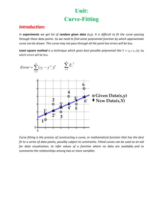
  • 1. Unit: Curve-Fitting Introduction: In experiments we get lot of random given data (x,y). It is difficult to fit the curve passing through these data points. So we need to find some polynomial function by which approximate curve can be drawn. This curve may not pass through all the point but errors will be less. Least square method is a technique which gives best possible polynomial like Y c + c (x). by which errors will be less. ' 2 1 ( ) n n i i i Error y y       n i i E 1 2 Curve fitting is the process of constructing a curve, or mathematical function that has the best fit to a series of data points, possibly subject to constraints. Fitted curves can be used as an aid for data visualization, to infer values of a function where no data are available, and to summarize the relationships among two or more variables
  • 2. A first degree polynomial equation: Yn c + c (x). A first degree polynomial equation is an exact fit through any two points with distinct x coordinates. A second degree polynomial: Yn c + c (x) + c (x)2 . Fitting a Line (first degree polynomial) equation: n= number of data points ∑ ∑ ∑ ∑ . ∑ OR Determinants: d=det d1= d2= Constants: c0=d1/d & c1=d2/d Fitting a Line : + (x). Problem: Using least square method Fit a line: Yn c + c (x) X 1 2 3 4 Y 2 6 12 20 Solution: n= number of data points=4 ∑ ∑ ∑ ∑ . ∑ X Y 1 2 1 2 2 3 4 12 3 12 9 36 4 20 16 80 ∑ =10 ∑ . 40 ∑ 30 ∑ 130
  • 3. OR Determinants: d=det 1 1 2 =20 d1= Dd2= =120 Constants: C0=d1/d = ‐ 5 and C1=d2/d=6 Best fitted line: + (X). ANSWER: + (X). Line Flowchart
  • 4. % LINE FITTING Yf=C0+C1(X) clc clear all %-------------Direct input of Data----------- x=[1 2 3 4]; y=[2 6 12 20]; n=length(x) %--------------OR-User UInput of data----- % n=input('Enter n='); % for i=1:n % fprintf('Enter x(%d)=',i); % x(i)=input(''); % fprintf('Enter y(%d)=',i); % y(i)=input(''); % end %-------------------------------------------- s1=sum(x); s2=sum(x.^2); s3=sum(y); s4=sum(x.*y); %-------------------------------------------- d=[n s1; s1 s2]; d1=[s3 s1; s4 s2]; d2=[n s3; s1 s4]; d=det(d); d1=det(d1); d2=det(d2); %-------------------------------------------- c0=d1/d; c1=d2/d; fprintf('BEST FIT ,Yn=%0.3f+%0.3f(X)n',c0,c1) %-------------------------------------------- yn=c0+c1*x; plot(x,y,'*',x,yn) %--------------------------------------------
  • 5. Solved Problems Fit the line yn=c0+c1*x x=[1 2 3 4]; y=[2 6 12 20]; ‐‐‐‐‐‐‐‐‐‐‐‐‐‐‐‐‐ X Y X2 XY ‐‐‐‐‐‐‐‐‐‐‐‐‐‐‐‐‐ 1 2 1 2 2 6 4 12 3 12 9 36 4 20 16 80 ‐‐‐‐‐‐‐‐‐‐‐‐‐‐‐‐‐ 10 40 30 130 Calculate d d1 d2 c 0 c1 by you BEST FIT ,Yn=‐5.000+6.000(X) Fit the line yn=c0+c1*x L=a0+a1T x=[ 20 30 40 50 60 70]; y=[800.3 800.4 800.6 800.7 800.9 801]; ‐‐‐‐‐‐‐‐‐‐‐‐‐‐‐‐‐‐‐‐‐‐‐ X Y X2 X.*Y ‐‐‐‐‐‐‐‐‐‐‐‐‐‐‐‐‐‐‐‐‐‐‐ 20 800 400 16006 30 800 900 24012 40 801 1600 32024 50 801 2500 40035 60 801 3600 48054 70 801 4900 56070 ‐‐‐‐‐‐‐‐‐‐‐‐‐‐‐‐‐‐‐‐‐‐‐‐‐‐‐‐‐ 270 4804 13900 216201 ‐‐‐‐‐‐‐‐‐‐‐‐‐‐‐‐‐‐‐‐‐‐‐‐‐‐‐‐‐ Calculate d d1 d2 c 0 c1 by you
  • 6. BEST FIT ,Yn=799.994+0.015(X) Fitting a second degree polynomial: + (X) + (X)2 ∑ ∑ ∑ ∑ ∑ ∑ ∑ ∑ 0 1 2 ∑ ∑ ∑ . 1 2 1 2 3 2 3 4 0 1 2 5 6 7 D det 1 2 1 2 3 2 3 4 D1 det 5 1 2 6 2 3 7 3 4 D2 Det 5 2 1 6 3 2 7 4 D3 Det 1 5 1 2 6 2 3 7 Constants: C0=d1/d , C1=d2/d and C2=d3/d Problem: Using least square method fit a second degree polynomial + (X) + (X)2 X 1 2 3 4 5 6 7 8 9 Y 2 6 7 8 10 11 11 10 9 Solution: ∑ ∑ ∑ ∑ ∑ ∑ ∑ ∑ ∑ ∑ ∑ = 0 1 2
  • 7. Table calculatins to be done by you X Y X2 X3 X4 XY XY2 S1 S5 S2 S3 S4 S6 S7 . 45 74 286 2025 15333 421 2771 On making table and solving S1 45, S2 286, S3 2025, S4 15333, s5 74 , s6 421, s7 2771, D det 166320 D1 det ‐154440 D2 Det D3 Det ‐44460 Constants: C0=D1/D = ‐0.9286 C1=D2/D= 3. C2=D3/D= ‐0.2673 Best fitted parabola: . .+3.523(X) 0.267(X)2
  • 8. Program % Quadratic FITTING Yf=C0+C1(X)+C2(x^2); % Quadratic FITTING Yf=C0+C1(X)+C2(x^2); clc clear all %‐‐‐‐‐‐‐‐‐‐‐‐‐‐‐‐‐‐‐‐‐‐‐‐‐‐‐‐‐‐‐‐‐‐‐‐‐‐‐‐‐‐‐‐‐‐‐‐‐‐‐‐‐‐ x=[1 2 3 4 5 6 7 8 9]; y=[2 6 7 8 10 11 11 10 9]; n=9; %‐‐‐‐‐‐‐‐‐‐‐‐‐‐‐‐‐‐‐‐‐‐‐‐‐‐‐‐‐‐‐‐‐‐‐‐‐‐‐‐‐‐‐‐‐‐‐‐‐‐‐‐‐‐ x2=x.^2; x3=x.^3; x4=x.^4; xy=x.*y; x2y=(x.^2).*y; s1=sum(x); s2=sum(x2); s3=sum(x3); s4=sum(x4); s5=sum(y); s6=sum(xy); s7=sum(x2y); %‐‐‐‐‐‐‐‐‐‐‐‐‐‐‐‐‐‐‐‐‐‐‐‐‐‐‐‐‐‐‐‐‐‐‐‐‐‐‐‐‐‐‐‐‐‐‐‐‐‐‐‐‐‐ d=[n s1 s2; s1 s2 s3 s2 s3 s4]; d1=[s5 s1 s2; s6 s2 s3 s7 s3 s4]; d2=[n s5 s2; s1 s6 s3 s2 s7 s4]; d3=[n s1 s5; s1 s2 s6 s2 s3 s7]; %‐‐‐‐‐‐‐‐‐‐‐‐‐‐‐‐‐‐‐‐‐‐‐‐‐‐‐‐‐‐‐‐‐‐‐‐‐‐‐‐‐‐‐‐‐‐‐‐‐‐‐‐‐‐ d=det(d); d1=det(d1); d2=det(d2); d3=det(d3); c0=d1/d; c1=d2/d; c2=d3/d; %‐‐‐‐‐‐‐‐‐‐‐‐‐‐‐‐‐‐‐‐‐‐‐‐‐‐‐‐‐‐‐‐‐‐‐‐‐‐‐‐‐‐‐‐‐‐‐‐‐‐‐‐‐‐ fprintf('BEST FIT ,Yn=%0.3f+%0.3f(X)+%0.3f(x^2)n',c0,c1,c2) %‐‐‐‐‐‐‐‐‐‐‐‐‐‐‐‐‐‐‐‐‐‐‐‐‐‐‐‐‐‐‐‐‐‐‐‐‐‐‐‐‐‐‐‐‐‐‐‐‐‐‐‐‐‐ yn=c0+c1*x+c2*x2; plot(x,y,'*',x,yn,'r') %‐‐‐‐‐‐‐‐‐‐‐‐‐‐‐‐‐‐‐‐‐‐‐‐‐‐‐‐‐‐‐‐‐‐‐‐‐‐‐‐‐‐‐‐‐‐‐‐‐‐‐‐‐‐‐‐‐‐‐‐‐‐‐‐‐‐‐‐‐‐‐‐‐‐‐‐‐‐‐‐‐‐‐‐ Option for i=1:n fprintf('%0.0f %0.0f %0.0f %0.0f %0.0f %0.0f %0.0f n',x(i),y(i),x2(i),x3(i),x4(i),xy(i),x2y(i)) end fprintf('‐‐‐‐‐‐‐‐‐‐‐‐‐‐‐‐‐‐‐‐‐‐‐‐‐‐‐‐‐‐‐‐‐‐‐‐‐‐‐‐‐‐‐‐‐‐‐‐‐‐‐‐‐‐‐‐‐‐‐‐‐‐‐‐‐‐‐‐‐‐‐‐ n'); fprintf('%0.0f %0.0f %0.0f %0.0f %0.0f %0.0f %0.0f n',s1, s5,s2,s3,s4,s6,s7)
  • 9. Solved Problem Fit the following quadratic/2nd degree/ parabolic curve + (X) + (X)2 x=[‐4 ‐3 ‐2 ‐1 0 1 2 3 4 5]; y=[21 12 4 1 2 7 15 30 45 67]; ‐‐‐‐‐‐‐‐‐‐‐‐‐‐‐‐‐‐‐‐‐‐‐‐‐‐‐‐‐‐‐‐‐‐‐‐‐‐‐ X Y x2 x3 x4 xy x2y ‐‐‐‐‐‐‐‐‐‐‐‐‐‐‐‐‐‐‐‐‐‐‐‐‐‐‐‐‐‐‐‐‐‐‐‐‐‐‐ ‐4 21 16 ‐64 256 ‐84 336 ‐3 12 9 ‐27 81 ‐36 108 ‐2 4 4 ‐8 16 ‐8 16 ‐1 1 1 ‐1 1 ‐1 1 0 2 0 0 0 0 0 1 7 1 1 1 7 7 2 15 4 8 16 30 60 3 30 9 27 81 90 270 4 45 16 64 256 180 720 5 67 25 125 625 335 1675 ‐‐‐‐‐‐‐‐‐‐‐‐‐‐‐‐‐‐‐‐‐‐‐‐‐‐‐‐‐‐‐‐‐‐‐‐‐‐ 5 204 85 125 1333 513 319 ‐‐‐‐‐‐‐‐‐‐‐‐‐‐‐‐‐‐‐‐‐‐‐‐‐‐‐‐‐‐‐‐‐‐‐‐‐‐ Remaining d d1 d2 d3 c0 c1 c3 …to be done by user
  • 10. Flowchart: Curve Fitting (Parabola) s1=sum(x); s2=sum(x.^2); s3=sum(x.^3); s4=sum(x.^4); s5=sum(y); s6=sum(x.*y); s7=sum((x.^2).*y); Calculation of Determinents d, d1, d2 c0=d1/d; c1=d2/d; c2=d3/d; Start Break Read x(i), y(i) For ( i=1 to n) Read n yf=c0+c1*x+c2*x.^2 Print C0, C1, C2 plot(x,y)
  • 11. Numerical Power For the power equation: PV^gamma =C P=[0.5 1 1.5 2 2.5 3]; V=[1.62 1 0.75 0.62 0.52 0.46]; Solution: Log(P)+ gamma*log(V)=log(C) Log(P)= log(C) - gamma *log(V) Y = C0 + C1 (X) C0=log(c) C1=-gamma Y=Log(P) X=Log(V) ------------------------------------------------------------------- V P X Y X^2 XY ------------------------------------------------------------------- 1.62 0.5 0.482426 -0.693147 0.232735 -0.334392 1.0 1.0 0. 0. 0. 0. 0.75 1.5 -0.287682 0.405465 0.082761 -0.116645 0.62 2. -0.478036 0.693147 0.228518 -0.331349 0.52 2.5 -0.653926 0.916291 0.427620 -0.599187 0.46 3. -0.776529 1.098612 0.602997 -0.853104 ----------------------------------------------------------- S1= -1.7137 S3=2.4204 S2=1.5746 S4=-2.2347 d = 6.5109 d1 =-0.0185 d2 = -9.2602 c0 =-0.0028 c1 = -1.4223 c = exp(c0)= 0.9972 gamma =-c1=1.4223 PV^1.422=0.997165
  • 12. Program Power clc clear all %‐‐‐‐‐‐‐‐‐‐‐‐‐Power Equation‐‐‐‐‐‐‐‐‐‐‐ %PV^Gamma=C p=[0.5 1.0 1.5 2.0 2.5 3.0]; v=[1.62 1.0 0.75 0.62 0.52 0.46]; n=6; y=log10(p); x=log10(v); xy=x.*y; x2=x.^2; s1=sum(x); s2=sum(x2); s3=sum(y); s4=sum(xy); %‐‐‐‐‐‐‐‐‐‐‐‐‐‐‐‐‐‐‐‐‐‐‐‐‐‐‐‐‐‐‐‐‐‐‐‐‐‐‐‐‐‐‐‐ d=n*s2‐s1*s1; d1=s3*s2‐s4*s1; d2=n*s4‐s1*s3; %‐‐‐‐‐‐‐‐‐‐‐‐‐‐‐‐‐‐‐‐‐‐‐‐‐‐‐‐‐‐‐‐‐‐‐‐‐‐‐‐‐‐‐‐ c0=d1/d; c1=d2/d; gamma=‐c1; c=exp(c0); %‐‐‐‐‐‐‐‐‐‐‐‐‐‐‐‐‐‐‐‐‐‐‐‐‐‐‐‐‐‐‐‐‐‐‐‐‐‐‐‐‐‐‐‐ fprintf('PV^%0.3f=%fn',gamma,c) %‐‐‐‐‐‐‐‐‐‐‐‐‐‐‐‐‐‐‐‐‐‐‐‐‐‐‐‐‐‐‐‐‐‐‐‐‐‐‐‐‐‐‐‐ %plot(p,v); for i=1:n fprintf('%f %f %f %f %f %f n',v(i),p(i),x(i),y(i),x2(i),xy(i)); end
  • 13. Numerical Exponential For the Exponential equation: y=aebx x=[2 4 6 8]; y=[25 38 56 84]; Solution y=aebx ln(y)=ln(a)+bx ln(e) Y =C0 +C1(x) yn=ln(y) C0=ln(a) C1=b ------------------------------------------------------ x y yn x^2 x*yn ------------------------------------------------------ 2. 25. 3.218876 4. 6.437752 4. 38. 3.637586 16. 14.550345 6. 56. 4.025352 36. 24.152110 8. 84. 4.430817 64. 35.446534 ----------------------------------------------------- S1=20 s3= 15.3126 s2= 120 s4=80.5867 d = 80 d1 = 225.7808 d2 = 16.0944 c0=2.8223 c1=0.2012 a=exp(c0)= 16.8148 b = c1=0.2012 y=16.815 e (0.2012x)
  • 14. Program Exponential clc clear all %‐‐‐‐‐‐‐‐‐‐‐‐‐Exponential‐‐‐‐‐‐‐‐‐‐‐ %y=ae^bx %‐‐‐‐‐‐‐‐‐‐‐‐‐‐‐‐‐‐‐‐‐‐‐‐‐‐‐‐‐‐‐‐‐‐‐‐‐‐‐‐‐‐‐‐ x=[2 4 6 8]; y=[25 38 56 84]; n=length(x); %‐‐‐‐‐‐‐‐‐‐‐‐‐‐‐‐‐‐‐‐‐‐‐‐‐‐‐‐‐‐‐‐‐‐‐‐‐‐‐‐‐‐‐‐ y1=log(y); %‐‐‐‐‐‐‐‐‐‐‐‐‐‐‐‐‐‐‐‐‐‐‐‐‐‐‐‐‐‐‐‐‐‐‐‐‐‐‐‐‐‐‐‐ x2=x.^2; xy1=x.*y1; s1=sum(x); s2=sum(x2); s3=sum(y1); s4=sum(xy1); %‐‐‐‐‐‐‐‐‐‐‐‐‐‐‐‐‐‐‐‐‐‐‐‐‐‐‐‐‐‐‐‐‐‐‐‐‐‐‐‐‐‐‐‐ d=n*s2‐s1*s1; d1=s3*s2‐s4*s1; d2=n*s4‐s1*s3; %‐‐‐‐‐‐‐‐‐‐‐‐‐‐‐‐‐‐‐‐‐‐‐‐‐‐‐‐‐‐‐‐‐‐‐‐‐‐‐‐‐‐‐‐ c0=d1/d; c1=d2/d; a=exp(c0); b=c1; %‐‐‐‐‐‐‐‐‐‐‐‐‐‐‐‐‐‐‐‐‐‐‐‐‐‐‐‐‐‐‐‐‐‐‐‐‐‐‐‐‐‐‐‐ fprintf('y=%0.3f e^(%0.3fx)n',a,b) %‐‐‐‐‐‐‐‐‐‐‐‐‐‐‐‐‐‐‐‐‐‐‐‐‐‐‐‐‐‐‐‐‐‐‐‐‐‐‐‐‐‐‐‐ for i=1:n fprintf('%f %f %f %f %f n',x(i),y(i),y1(i),x2(i),xy1(i)); end
  • 15. Solver :% POLYFIT clear all x=[19 25 30 36 40 45 50]; y=[76 77 79 80 82 83 85]; d=1; %d=1 (line) d=2(parabola) c=polyfit(x,y,d) % yn = polyval(c, x); yn=c(2)+c(1)*x; plot(x,y,'*',x,yn)