
Recommended
Recommended
More Related Content
What's hot
What's hot (19)
Similar to Mayo Slides: Part I Meeting #2 (Phil 6334/Econ 6614)
Similar to Mayo Slides: Part I Meeting #2 (Phil 6334/Econ 6614) (20)
More from jemille6
More from jemille6 (20)
Recently uploaded
Recently uploaded (20)
Mayo Slides: Part I Meeting #2 (Phil 6334/Econ 6614)
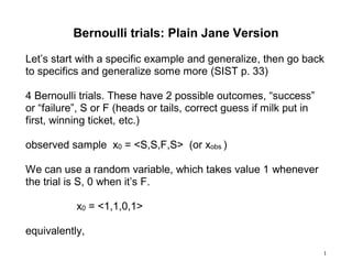
- 1. 1 Bernoulli trials: Plain Jane Version Let’s start with a specific example and generalize, then go back to specifics and generalize some more (SIST p. 33) 4 Bernoulli trials. These have 2 possible outcomes, “success” or “failure”, S or F (heads or tails, correct guess if milk put in first, winning ticket, etc.) observed sample x0 = <S,S,F,S> (or xobs ) We can use a random variable, which takes value 1 whenever the trial is S, 0 when it’s F. x0 = <1,1,0,1> equivalently,
- 2. 2 x0 = <X1=1, X2 =1, X3=0, X1=1> Let Pr(X = 1) = 𝜃 for any trial, and that trials are independent 𝜃 a parameter; in the Bernoulli case it’s from 0 to 1 If we knew 𝜃, if we could compute Pr(x0; 𝜃) = Pr(observed x0; assuming prob of success at each trial = 𝜃) f(x0; 𝜃)
- 3. 3 The joint outcome involves series of “ands” x0 = the 1st trial is 1 and 2nd trial is 1 and 3rd trial is 0 and 4th trial is 1 So, Pr(x0; 𝜃) = Pr (X1 = 1 and X2 = 1 and X3 = 0 and X4 = 1; 𝜃) Because the trials are independent, the probability multiplies Pr(x0; 𝜃) = Pr(X1 = 1; 𝜃)Pr (X2 = 1; 𝜃)Pr (X3 = 0; 𝜃)Pr (X4 = 1; 𝜃) Suppose 𝜃 = .2 (as in Royall’s example)
- 4. 4 (e.g., 100 balls, 20 are red and we randomly draw, and success is getting a red ball) What’s Pr(X = 1) assuming the probability of X = 1 is .2 ? Who is buried in Grant’s tomb? Therefore, Lik(𝜃 = .2; x0) = Pr( 1,1,0,1; .2) = (.2)(.2)(.8)(.2) Where did .8 come from? If Pr(S = .2) then Pr(not-S) = .8 (since by the axioms, Pr( S or ~S) = 1 = Pr(S) + Pr (~S)) Note SIST error last line p. 33, it should be Lik(.2) because Royall is about to use H0: 𝜃 ≤ .2 vs H1: 𝜃 > .2 to compare his likelihoodist inference with the frequentist significance test
- 5. 5 We want to compare Lik(𝜃 = .2; x0) with the likelihood given 𝜃 = .8 (measure of comparative “support”) Lik(𝜃 = .8; x0) = Pr( 1,1,0,1; .8) = (. )(. )(. )(. ) .0064 vs. .1024 In general, with this x0, Lik(𝜃; x0) = Pr( 1,1,0,1; 𝜃) = (𝜃)( 𝜃)(1 - 𝜃)( 𝜃) = 𝜃3 (1 - 𝜃) order doesn’t matter So Lik(𝜃 = .2; x0) = Pr( 1,1,0,1; .2) = (.2)(.2)(.8)(.2) and Lik(𝜃 = .8; x0) = Pr( 1,1,0,1; .8) = (.8)(.8)(.2)(.8) LR (𝜃 = .2 over 𝜃 = .8) = .0064 / .1024
- 6. 6 (.2)3 (.8)/ (.8)3 (.2) = (.25)3 (4) ~.06 Can also write the LR reverse LR (𝜃 = .8 over 𝜃 = .2) = 16.6
- 7. 7 It’s useful to start with the Likelihoodist, because it’s a key example of a logic of (comparative) evidence, and hits one of the big “wars” Still we don’t usually crank out numbers; My book does because it’s taking the criticisms in their actual location and the people arguing use numbers
- 8. 8 The book asks the reader to find Lik( .75) with the same outcome <1,1,0,1> (note .75 is closer to .8 than to .2 so .8 is more likely) This is the maximally likely 𝜃 as the observed proportion is ¾ What’s Lik(.75; x0)?
- 9. 9 .1054
- 10. 10 Generalize for 4 Bernoulli trials More generally, still for 4 trials, say we don’t know the result, Write the result of the kth trial is xk as Xk = xk Random variable, capital Xk and lower case xk is its value xobs = (X1 = x1 and X2 = x2 and X3 = x3 and X4 = x4 ) Pr(x; 𝜃) = Pr(x1; 𝜃)Pr(x2; 𝜃)Pr (x3; 𝜃) Pr (x4; 𝜃) These should really be frequency distributions: f(x1; 𝜃) f(x2; 𝜃) f(x3; 𝜃) f(x4; 𝜃)
- 11. 11 Shortcut abbreviation for multiplying: f(x1; 𝜃) f(x2; 𝜃) f(x3; 𝜃) f(x4; 𝜃) ∏ 𝑓(𝑥 𝑘; 𝜃) 4 𝑘=1
- 12. 12 Now take the Royall example on p. 34, n = 17, there are 9 successes and 8 failures (ugly numbers, they’re his) Lik(x; θ) = θ9 (1 –θ)8 Observed proportion of successes = .53 Even without calculating, θ = .53 makes the observed outcome most probable, it’s the maximally likely θ value
- 13. 13 He fixes θ = .2 and considers the Likelihood ratio of .2 and various alternatives Since the sample proportion is .53, any value of θ further from .53 than .2 is will be less well supported than .2 Start with .2, .33 more takes us to .53, another .33 goes to .86 So any θ > .86 is less likely than is .2 Likelihood ratio of .2 and .9 LR (θ = .2 over θ = .9) = [.29 (.8)8 ]/[ [.99 (.1)8 ] = 22.2 (top p. 36)
- 14. 14 both are too hideously small, we would never be computing them. But we can group (2/9)9 (8)8 ~ 22 top of p. 36
- 15. 15 Royall: “Because H0: θ ≤ .2 contains some simple hypotheses that are better supported than some hypotheses in H1 (e.g., θ = .2 is better supported than θ = .9)…the law of likelihood does not allow the characterization of these observations as strong evidence for H1 over H0 . The significance tester tests H0: θ ≤ .2 vs. H1: θ > .2 So he rules out composite hypotheses.
- 16. 16 The significance tester tests H0: θ ≤ .2 vs. H1: θ > .2 She would reject H0 and infer some (pos) discrepancy from .2 (observed mean M – expected mean under H0) in standard deviation or standard error units (.53 - .2)/.1 ~ 3.3 Here 1 SE is .1 Test Statistic d(x0) is (.53 - .2)/.1
- 17. 17 Lets us use the Standard Normal curve (we’re using a Normal approximation) (area to the right of 3) ~0, very significant. Pr(d(X) ≥ d(x0); H0) ~ .003
- 18. 18 Pr(d(X) < d(x0); H0) ~ .997 (see p. 35) Admittedly, just reporting there’s evidence H1: θ > .2, as our significance tester, doesn’t seem so informative either. In inferring H1, she is only inferring some positive discrepancy from .3 A 95 % confidence interval estimate, which we have not discussed, would be .53 ± 2SE [.33 < θ < .73] We’ll see how severity also gives a report of discrepancy and has some advantages.
- 19. 19 The Likelihoodist gives a series of comparisons: this is better supported than that, less strongly than some other value. If you give enough comparisons, maybe our inferences aren’t so different. Is this really a statistical inference? Or just a report of the data? For the Likelihoodist it is, and the fact that a significance test is not comparative even precludes it from being a proper measure of evidence.
- 20. 20 One Stat War Explained Likelihoodists maintain that any genuine test or “rule of rejection” should be restricted to comparing the likelihood of H versus some point alternative H′ relative to fixed data x No wonder the Likelihoodist disagrees with the significance tester. Elliott Sober: “The fact that significance tests don’t contrast the null with alternatives suffices to show that they do not provide a good rule for rejection” (Sober 2008, p. 56). The significance test has an alternative H1: θ > 0.2! (not a point) (STINT p. 35)
- 21. 21 While we’re at notation: let’s generalize for n Bernoulli trials xobs a member of the sample space: xobs ε R real numbers) xobs = X1 = x1 and X2 = x2 and X3 = x3 ….and Xn = xn Pr(xobs; 𝜃) = f(x1; 𝜃) f(x2; 𝜃) f(x3; 𝜃) …f(xn; 𝜃) Shortcut abbreviation: ∏ 𝑓(𝑥 𝑘; 𝜃) 𝑛 𝑘=1
- 22. 22 ∏ 𝑓(𝑥 𝑘; 𝜃) 𝑛 𝑘=1 I’ve run out of letters, let z = number of success out of n, n – k failures Lik(x; θ) θz (1 –θ)n-z More notation z = ∑ 𝑥 𝑘 𝑛 𝑘=1
- 23. 23 See the comparison in Souvenir B, likelihood vs error statistical p. 41 Spanos manuscript chapter 2: 19-21, set theoretic observations End Part I of Mayo
- 24. 24