SlideShare una empresa de Scribd logo
1 de 70
Descargar para leer sin conexión
Engineering Circuit Analysis, 7th Edition

1.

Chapter Fifteen Solutions

10 March 2006

Note that iL(0+) = 12 mA. We have two choices for inductor model:

= 0.032s Ω
0.032s Ω
= 384 μV

12
mA
s

PROPRIETARY MATERIAL. © 2007 The McGraw-Hill Companies, Inc. Limited distribution permitted only to teachers
and educators for course preparation. If you are a student using this Manual, you are using it without permission.
Engineering Circuit Analysis, 7th Edition

2.

Chapter Fifteen Solutions

10 March 2006

iL(0-) = 0, vC(0+) = 7.2 V (‘+’ reference on left). There are two possible circuits, since
the inductor is modeled simply as an impedance:
1
Ω
0.002s

73 Ω

1
Ω
0.002s

7.2
V
s
0.03s Ω

73 Ω

+
V(s)
-

14.4 mA
0.03s Ω

+
V(s)
-

PROPRIETARY MATERIAL. © 2007 The McGraw-Hill Companies, Inc. Limited distribution permitted only to teachers
and educators for course preparation. If you are a student using this Manual, you are using it without permission.
Engineering Circuit Analysis, 7th Edition

Chapter Fifteen Solutions

10 March 2006

3.
(a)

Z m (s) =

2s
2000 / s
20s
1000
+
=
+
20 + 0.1s 2 + 1000 / s s + 200 s + 500

20s 2 + 10, 000s + 1000s + 200, 000
=
=
s 2 + 700s + 100, 000

(b)

Zin(-80) = - 10.95 Ω

(c)

Zin ( j80) =

(d)

YRL =

1 10 s + 200
+
=
20 s
20s

(e)

YRC =

20s 2 + 11, 000s + 200, 000
s 2 + 700s + 100, 000

1
s + 500
+ 0.001s =
2
1000

(f)

−128, 000 + j880, 000 + 200, 000
= 8.095∠54.43° Ω
−6400 + j 56, 000 + 100, 000

s + 200
+ 0.5 + 0.001s
YRL + YRC
s + 200 + 10s + 0.02s 2
= 20s
=
(s + 200)
YRL YRC
0.001s 2 + 0.7s + 100
(0.001s + 0.5)
20s
20s 2 + 11, 000s + 200, 000
=
= Z(s)
s 2 + 700s + 100, 000

PROPRIETARY MATERIAL. © 2007 The McGraw-Hill Companies, Inc. Limited distribution permitted only to teachers
and educators for course preparation. If you are a student using this Manual, you are using it without permission.
Engineering Circuit Analysis, 7th Edition

Chapter Fifteen Solutions

10 March 2006

4.

1
2 × 10⁻³ s

1
2 × 10⁻³ s

1
1
⎛
⎞ ⎛
⎞
Zin = ⎜ 20 +
= (20 + 500s-1) || (40 + 500s-1)
|| ⎜ 40 +
−3 ⎟
−3 ⎟
2 × 10 s ⎠ ⎝
2 × 10 s ⎠
⎝

=

80s 2 + 3000s +25000
6s 2 + 100s

PROPRIETARY MATERIAL. © 2007 The McGraw-Hill Companies, Inc. Limited distribution permitted only to teachers
and educators for course preparation. If you are a student using this Manual, you are using it without permission.
Engineering Circuit Analysis, 7th Edition

Zin =

Zin ( j8) =

(c)

Zin (−2 + j 6) =

(d)

(e)

10 March 2006

50 16(0.2s) 50
16s
16s 2 + 50s + 4000
+
=
+
=
s 16 + 0.2s
s s + 80
s 2 + 80s

(a)

(b)

5.

Chapter Fifteen Solutions

−1024 + 4000 + j 400
= 0.15842 − j 4.666 Ω
−64 + j 640

16(4 − 36 − j 24) − 100 + j 300 + 4000
= 6.850∠ − 114.3° Ω
−32 − j 24 − 160 + j 480

0.2 sR
50
0.2Rs 2 + 10s + 50R
,
+
=
s R + 0.2s
0.2s 2 + Rs
5R − 50 + 50 R
Zin (−5) =
∴ 55R = 50, R = 0.9091 Ω
5 − 5R
Zin =

R = 1Ω

PROPRIETARY MATERIAL. © 2007 The McGraw-Hill Companies, Inc. Limited distribution permitted only to teachers
and educators for course preparation. If you are a student using this Manual, you are using it without permission.
Engineering Circuit Analysis, 7th Edition

6.

2 mF →

Chapter Fifteen Solutions

10 March 2006

1
Ω, 1 mH → 0.001s Ω,
2 × 10⁻³ s

Zin = (55 + 500/ s) || (100 + s/ 1000) =
s ⎞
500 ⎞ ⎛
⎛
⎟
⎜ 55 +
⎟ ⎜100 +
55s 2 + 5.5005 × 10⁶ s + 5 × 10⁷
s ⎠ ⎝
1000 ⎠
⎝
=
s
500
s 2 + 5 × 10⁵ s + 1.55 × 10⁵
155 +
+
s
1000

PROPRIETARY MATERIAL. © 2007 The McGraw-Hill Companies, Inc. Limited distribution permitted only to teachers
and educators for course preparation. If you are a student using this Manual, you are using it without permission.
Engineering Circuit Analysis, 7th Edition

7.

Chapter Fifteen Solutions

10 March 2006

We convert the circuit to the s-domain:
1/sCμ Ω

Vπ
1/sCπ Ω

Vπ

rπ R B
and
rπ + R B + rπ R BCπ s
ZL = RC || RL = RCRL/ (RC + RL), we next connect a 1-A source to the input and write two
nodal equations:

Defining Zπ = RB || rπ || (1/sCπ) =

1
Solving,
Vπ =

= Vπ/ Zπ + (Vπ – VL)Cμ s

-gmVπ = VL/ ZL + (VL – Vπ)Cμ s

[1]
[2]

rπ R B (1 + Z L C μ s )
Z L rπ R BCπ C μ s 2 + (g m Z L rπ R BC μ + rπ R BCπ + rπ R BC μ + Z L rπ C μ +Z L R BC μ )s + rπ + R B

Since we used a 1-A ‘test’ source, this is the input impedance. Setting both capacitors to
zero results in rπ || RB as expected.

PROPRIETARY MATERIAL. © 2007 The McGraw-Hill Companies, Inc. Limited distribution permitted only to teachers
and educators for course preparation. If you are a student using this Manual, you are using it without permission.
Engineering Circuit Analysis, 7th Edition

8.
0.115s Ω

Chapter Fifteen Solutions

10 March 2006

460 μV

I

2
s

V

2
+ 460 × 10−6
2.162
9400
s
+
=
V(s) = 4700
0.115s + 4700
s (0.115s + 4700)
4700 + 0.115s

=

18.8
81740
18.8
a
b
+
=
+
+
s + 40870
s (s + 40870)
s + 40870
s
s + 40870

where a =

Thus, V(s) =

81740
s + 40870

= 2 and b =
s =0

81740
s

= -2
s = -40870

18.8
2
2
. Taking the inverse transform of each term,
+
s + 40870
s s + 40870

v(t) = [16.8 e-40870t + 2] u(t) V

PROPRIETARY MATERIAL. © 2007 The McGraw-Hill Companies, Inc. Limited distribution permitted only to teachers
and educators for course preparation. If you are a student using this Manual, you are using it without permission.
Engineering Circuit Analysis, 7th Edition

9.

Chapter Fifteen Solutions

10 March 2006

v(0-) = 4 V

303030
Ω
s
9
s

4
V
s

I(s)

9 4
−
5
4.545 × 10⁻⁶
s s
=
=
I(s) =
303030
s +0.2755
1.1 × 10⁶ + 303030
+ 1.1 × 10⁶
s
Taking the inverse transform, we find that i(t) = 4.545 e-0.2755t u(t) μA

PROPRIETARY MATERIAL. © 2007 The McGraw-Hill Companies, Inc. Limited distribution permitted only to teachers
and educators for course preparation. If you are a student using this Manual, you are using it without permission.
Engineering Circuit Analysis, 7th Edition

10.

Chapter Fifteen Solutions

10 March 2006

From the information provided, we assume no initial energy stored in the inductor.
(a) Replace the 100 mH inductor with a 0.1s-Ω impedance, and the current source with a
25 × 10−6
A source.
s
0.1s Ω
25
s

V

25 × 10−6 ⎡ 2 (0.1s) ⎤
5 × 10⁻⁶
5 × 10-5
=
=
V
⎢ 2 + 0.1s ⎥
0.1s + 2
s
s + 20
⎣
⎦
Taking the inverse transform,

(b) V(s) =

v(t) = 50 e-20t mV

The power absorbed in the resistor R is then p(t) = 0.5 v2(t) = 1.25 e-40t nW

PROPRIETARY MATERIAL. © 2007 The McGraw-Hill Companies, Inc. Limited distribution permitted only to teachers
and educators for course preparation. If you are a student using this Manual, you are using it without permission.
Engineering Circuit Analysis, 7th Edition

11.

Chapter Fifteen Solutions

10 March 2006

We transform the circuit into the s-domain, noting the initial condition of the capacitor:
V1

V2

4/s Ω

2/s

6/s

2/s V

Writing our nodal equations,
V1 − 2

s + V1 − V2 +
1
1
2

V1 + 2
4

s =0

[1]

s

V2 − V1 V2
+
=6
1
1
2

[2]

We may solve to obtain

V1 =

and

V1 =

Taking the inverse transforms,
and

−6 ( s − 12 )
s ( 3s + 20 )
2 ( s + 44 )

s ( 3s + 20 )

=

3.6
−5.6
+
s + 6.67 s

=

−3.73 4.4
+
s + 6.67
s

v1(t) = –5.6e–6.67t + 3.6 V, t ≥ 0
v2(t) = –3.73e–6.67t + 4.4 V, t ≥ 0

PROPRIETARY MATERIAL. © 2007 The McGraw-Hill Companies, Inc. Limited distribution permitted only to teachers
and educators for course preparation. If you are a student using this Manual, you are using it without permission.
Engineering Circuit Analysis, 7th Edition

12.

Chapter Fifteen Solutions

10 March 2006

We transform the circuit into the s-domain, noting the initial condition of the inductor:

V1

V2

(a) Writing our nodal equations,
4V1 − 3V2 =

and
−3V1 + 3V2 +

2
s

[1]

2/s

4/s A

36 V

V2 + 36 4
=
9s
s

or

9s Ω

[2]

1⎞
⎛
−3V1 + ⎜ 3 + ⎟ V2 = 0
9s ⎠
⎝

We may solve to obtain

and

⎛
⎞
⎜ 1 ⎟ 1 ⎛1⎞
3
V1 =
= ⎜
⎟+ ⎜ ⎟
s ( 27s + 4 ) 2 ⎜ s + 4 ⎟ 2 ⎝ s ⎠
27 ⎠
⎝
54
2
=
V2 =
27s + 4 s + 4
27

Taking the inverse transforms,
and

2 ( 27s + 1)

v1(t) = 1.5–0.1481t + 0.5 V, t ≥ 0
v2(t) = 2e–0.1481t V, t ≥ 0

(b)

PROPRIETARY MATERIAL. © 2007 The McGraw-Hill Companies, Inc. Limited distribution permitted only to teachers
and educators for course preparation. If you are a student using this Manual, you are using it without permission.
Engineering Circuit Analysis, 7th Edition

13.

Chapter Fifteen Solutions

10 March 2006

(a) We transform the circuit into the s-domain, noting the initial condition of the
capacitor:

1/s Ω
12/s

I2

I1

9/s V

Writing the two required mesh equations:
1⎞
1
3
⎛
⎜ 6 + ⎟ I1 − I 2 =
s⎠
s
s
⎝
1
1⎞
9
⎛
− I1 + ⎜12 + ⎟ I 2 =
s
s⎠
s
⎝

[1]
[2]

⎛
⎞
2 ⎡ ( 3s + 1) ⎤ 2 1 ⎜ 1 ⎟
Solving yields I1 = ⎢
⎥= −
3 ⎢ s ( 4s + 1) ⎥ 3s 6 ⎜ s + 1 ⎟
⎣
⎦
4⎠
⎝
1 ⎡ ( 9s + 2 ) ⎤ 2 1 ⎛ 1 ⎞
⎟
and I 2 = ⎢
⎥= + ⎜
3 ⎢ s ( 4s + 1) ⎥ 3s 12 ⎜ s + 1 ⎟
⎣
⎦
4⎠
⎝
Thus, taking the inverse Laplace transform, we obtain
i1 (t ) =

2 1 −t4
− e A, t ≥ 0
3 6

and

i2 (t ) =

2 1 − t4
+ e A, t ≥ 0
3 12

(b)

PROPRIETARY MATERIAL. © 2007 The McGraw-Hill Companies, Inc. Limited distribution permitted only to teachers
and educators for course preparation. If you are a student using this Manual, you are using it without permission.
Engineering Circuit Analysis, 7th Edition

14.

Chapter Fifteen Solutions

10 March 2006

(a) We transform the circuit into the s-domain, noting the initial condition of the
inductor:
I1

9/s

sΩ

I2

8V

Writing the two required mesh equations:
9
+8
s
−sI1 + (10 + s ) I 2 = −8

( 2 + s ) I1 − sI 2 =

[1]
[2]

⎡
⎤
1 ⎢ ( 89s + 90 ) ⎥ 35 ⎛ 1 ⎞ 4.5
⎟+
Solving yields I1 =
= ⎜
12 ⎢ s s + 5 ⎥ 12 ⎜ s + 5 ⎟ s
3⎠
⎢
⎝
3 ⎥
⎣
⎦
⎡
⎤
⎛
⎞
−7 ⎢ 1
⎥=− 7 ⎜ 1 ⎟
and I 2 =
12 ⎢ s + 5 ⎥
12 ⎜ s + 5 ⎟
3⎠
⎢
⎝
3 ⎥
⎣
⎦

(

(

)

)

Thus, taking the inverse Laplace transform, we obtain
i1 (t ) =

35 −1.667 t
e
+ 4.5 A, t ≥ 0
12

and

i2 (t ) = −

7 −1.667 t
A, t ≥ 0
e
12

(b)

PROPRIETARY MATERIAL. © 2007 The McGraw-Hill Companies, Inc. Limited distribution permitted only to teachers
and educators for course preparation. If you are a student using this Manual, you are using it without permission.
Engineering Circuit Analysis, 7th Edition

15.

Chapter Fifteen Solutions

10 March 2006

v(t) = 10e-2t cos (10t + 30o) V

scos30o -10sin30o
0.866s - 5
cos (10t + 30 ) ⇔
= 2
2
s +100
s + 100
-at
L {f(t)e } ⇔ F(s + a), so
o

V(s) = 10

0.866 ( s + 2 ) - 5

(s + 2)

2

+ 100

=

8.66s - 16.34
s + 100

The voltage across the 5-Ω resistor may be found by simple voltage division. We first
50
Ω. Thus,
note that Zeff = (10/s) || 5 =
5s + 10
⎛ 50 ⎞
⎜
⎟ Vs
50 Vs
50 Vs
⎝ 5s + 10 ⎠
=
=
V5Ω =
2
⎛ 50 ⎞
( 0.5s + 5) ( 5s + 10 ) + 50 2.5s + 30s + 100
0.5s + 5 + ⎜
⎟
⎝ 5s + 10 ⎠
V
0.866s - 3.268
34.64s - 130.7
=
(a) Ix = eff = 40
2
2
5
⎡( s + 2 ) + 100 ⎤ ⎡s 2 + 12s + 40 ⎤
⎡( s + 2 ) + 100 ⎤ ⎡( s + 6 )2 + 100 ⎤
⎣
⎦
⎣
⎦
⎦
⎣
⎦⎣

(b) Taking the inverse transform using MATLAB, we find that
ix(t) = e-6t [0.0915cos 2t - 1.5245 sin 2t] - e-2t [0.0915 cos10t - 0.3415 sin 10t] A

PROPRIETARY MATERIAL. © 2007 The McGraw-Hill Companies, Inc. Limited distribution permitted only to teachers
and educators for course preparation. If you are a student using this Manual, you are using it without permission.
Engineering Circuit Analysis, 7th Edition

16.

VC1

10 March 2006

2
Ω V2
s

V1
3
s

Chapter Fifteen Solutions

5
Ω
s

8s Ω

5
V
s

Node 1:

0 = 0.2 (V1 – 3/ s) + 0.2 V1 s + 0.5 (V1 – V2) s

Node 2:

0 = 0.5 (V2 – V1) s + 0.125 V2 s + 0.1 (V2 + 5/ s)

Rewriting, (3.5 s 2 + s) V1 + 2.5 s 2 V2 = 3
-4 s 2 V1 + (4 s 2 + 0.8 s + 1) V2 = -4

[1]
[2]

Solving using MATLAB or substitution, we find that
−20s 2 + 16s + 20
40s 4 + 68s3 + 43s 2 + 10s
−20s 2 + 16s + 20
⎛ 1 ⎞
= ⎜ ⎟
⎝ 40 ⎠ s ( s + 0.5457 - j 0.3361)( s + 0.5457 + j 0.3361)( s + 0.6086 )

V1 (s) =

which can be expanded:
a
b
b*
c
V1 (s) =
+
+
+
s
s + 0.5457 - j 0.3361 s + 0.5457 + j 0.3361 s + 0.6086
Using the method of residues, we find that
a = 2, b = 2.511 ∠101.5o, b* = 2.511∠-101.5o and c = -1.003.
Thus,taking the inverse transform,
v1(t) = [2 – 1.003 e-0.6086t + 5.022 e-0.5457t cos (0.3361t – 101.5o)] u(t) V

PROPRIETARY MATERIAL. © 2007 The McGraw-Hill Companies, Inc. Limited distribution permitted only to teachers
and educators for course preparation. If you are a student using this Manual, you are using it without permission.
Engineering Circuit Analysis, 7th Edition

17.

Chapter Fifteen Solutions

10 March 2006

With zero initial energy, we may draw the following circuit:
2 s-1 Ω

3
V
s

5 s-1 Ω

8sΩ

5
V
s

Define three clockwise mesh currents I1, I2, and I3 in the left, centre and right meshes,
respectively.
Mesh 1: -3/s + 5I1 + (5/s)I1 – (5/s)I2 = 0
Mesh 2: -(5/s)I1 + (8s + 7/s)I2 – 8s I3 = 0
Mesh 3: -8sI2 + (8s + 10)I3 – 5/s = 0
Rewriting,
(5s + 5) I1 – 5 I2
-5 I1
+ (8s2 +7) I2 – 8s2 I3
- 8s2 I2 + (8s2 + 10s) I3

= 3
= 0
= 5

[1]
[2]
[3]

Solving, we find that
I2(s) =
=

2

20s + 32s + 15
20s 2 + 32s + 15
=⎛ 1 ⎞
⎜ ⎟
2
40s + 68s + 43s + 10 ⎝ 40 ⎠ ( s + 0.6086 )( s + 0.5457 - j 0.3361)( s + 0.5457 + j 0.3361)
3

a
b
b*
+
+
( s + 0.6086 ) ( s + 0.5457 - j 0.3361) ( s + 0.5457 + j 0.3361)

where a = 0.6269, b = 0.3953∠-99.25o, and b* = 0.3955∠+99.25o
Taking the inverse tranform, we find that
o
o
i2(t) = [0.6271e-0.6086t + 0.3953e-j99.25 e(-0.5457 + j0.3361)t + 0.3953ej99.25 e(-0.5457 - j0.3361)t ]u(t)
= [0.6271e-0.6086t + 0.7906 e-0.5457t cos(0.3361t + 99.25o)] u(t)

PROPRIETARY MATERIAL. © 2007 The McGraw-Hill Companies, Inc. Limited distribution permitted only to teachers
and educators for course preparation. If you are a student using this Manual, you are using it without permission.
Engineering Circuit Analysis, 7th Edition

18.

Chapter Fifteen Solutions

10 March 2006

We choose to represent the initial energy stored in the capacitor with a current source:
V1
3
V
s

5
Ω
s

•

2
Ω
s

↑ 1.8 A

V2
5
V
s

8s Ω

•

Node 1:

Node 2:
Rewriting,

3
s + s V + s (V - V )
1.8 =
1
1
2
5
5
2
5
V2 +
1
s
s
0 =
(V2 - V1 ) +
V2 +
2
8s
10
V1 -

(5s2 + 4s) V1 – 5s2 V2 = 18s + 6
-4s2 V1 + (4s2 + 0.8s + 1)V2 = -4

Solving, we find that V1(s) =

[1]
[2]

360s3 + 92s 2 + 114s + 30
s(40s3 + 68s 2 + 43s + 10)

a
b
c
c*
+
+
+
=
s
s + 0.6086 s + 0.5457 - j 0.3361 s + 0.5457 + j 0.3361
where a = 3, b = 30.37, c = 16.84 ∠136.3o and c* = 16.84 ∠-136.3o
Taking the inverse transform, we find that
o
v1(t) = [3 + 30.37e-0.6086t + 16.84 ej136.3 e-0.5457t ej0.3361t
o
+ 16.84 e-j136.3 e-0.5457t e-j0.3361t ]u(t) V
= [3 + 30.37e-0.6086t + 33.68e-0.5457t cos (0.3361t + 136.3o]u(t) V

PROPRIETARY MATERIAL. © 2007 The McGraw-Hill Companies, Inc. Limited distribution permitted only to teachers
and educators for course preparation. If you are a student using this Manual, you are using it without permission.
Engineering Circuit Analysis, 7th Edition

19.

Chapter Fifteen Solutions

10 March 2006

We begin by assuming no initial energy in the circuit and transforming to the s-domain:
V1
20

10
Ω
s
2s Ω

s+3
A
(s + 3) 2 + 16

(a) via nodal analysis, we write:
V
20s + 60
s
=
( V1 - Vx ) + 1
2
(s + 3) + 16
10
5
V
120
s
= x +
( Vx − V1 )
2
(s + 3) + 16
2s
10

Vx

30

4
A
(s + 3)2 + 16

[1] and
[2]

Collecting terms and solving for Vx(s), we find that
Vx(s) =
=

200s(s 2 + 9s + 12)
2s 4 + 17s3 + 90s 2 + 185s + 250
200s(s 2 + 9s + 12)
( s + 3 - j 4 )( s + 3 + j 4 )( s + 1.25 - j1.854 )( s + 1.25 + j1.854 )

(b) Using the method of residues, this function may be rewritten as
a
a*
b
b*
+
+
+
( s + 3 - j 4 ) ( s + 3 + j 4 ) ( s + 1.25 - j1.854 ) ( s + 1.25 + j1.854 )

with a = 92.57 ∠ -47.58o, a* = 92.57 ∠ 47.58o, b = 43.14 ∠106.8o, b* = 43.14 ∠-106.8o
Taking the inverse transform, then, yields
o

o

vx(t) = [92.57 e-j47.58 e-3t ej4t + 92.57 ej47.58 e-3t e-j4t
o
o
+ 43.14ej106.8 e-1.25t ej1.854t + 43.14e-j106.8 e-1.25t e-j1.854t] u(t)

= [185.1 e-3t cos (4t - 47.58o) + 86.28 e-1.25t cos (1.854t + 106.8o)] u(t)

PROPRIETARY MATERIAL. © 2007 The McGraw-Hill Companies, Inc. Limited distribution permitted only to teachers
and educators for course preparation. If you are a student using this Manual, you are using it without permission.
Engineering Circuit Analysis, 7th Edition

20.

Chapter Fifteen Solutions

10 March 2006

We model the initial energy in the capacitor as a 75-μA independent current source:

0.005s Ω
162.6s
V
s 2 + 4π 2

106
Ω
s

First, define Zeff = 106/s || 0.005s || 20 =

↑

V

75 μA

s
Ω
10 s + 0.005s + 200
-6 2

Then, writing a single KCL equation, 75 ×10-6 =

V (s)
1 ⎛
162.6s ⎞
+
⎜ V (s) - 2
⎟
Zeff
20 ⎝
s + 4π 2 ⎠

which may be solved for V(s):
V(s) =
=

75s ( s 2 + 1.084 × 10⁵s + 39.48 )
s 4 + 5.5 × 10⁴s3 + 2 × 10⁸s 2 + 2.171× 10⁶s + 7.896 × 10⁹
75s s 2 + 1.084 ×10⁵s + 12.57

(

)

( s + 51085)( s + 3915)( s - j 6.283)( s + j 6.283)

(NOTE: factored with higher-precision denominator coefficients using MATLAB to
obtain accurate complex poles: otherwise, numerical error led to an exponentially
growing pole i.e. real part of the pole was positive)
a
b
c
c*
=
+
+
+
( s + 51085 ) ( s + 3915 ) ( s - j 2π ) ( s + j 2π )
where a = -91.13, b = 166.1, c = 0.1277∠89.91o and c* = 0.1277∠-89.91o.
Thus, consolidating the complex exponential terms (the imaginary components cancel),
v(t) = [-91.13e-51085t + 166.1e-3915t + 0.2554 cos (2πt + 89.91o)] u(t) V
(b) The steady-state voltage across the capacitor is V = [255.4 cos(2πt + 89.91o)] mV
This can be written in phasor notation as 0.2554 ∠89.91o V. The impedance across
which this appears is Zeff = [jωC + 1/jωL + 1/20]-1 = 0.03142 ∠89.91o Ω, so
Isource = V/ Zeff = 8.129∠-89.91o A.
Thus, isource = 8.129 cos 2πt A.
(c) By phasor analysis, we can use simple voltage division to find the voltage division to
find the capacitor voltage:
(162.6∠0 ) ( 0.03142∠89.91o )
VC(jω) =
= 0.2554∠89.92o V which agrees with
20 + 0.03142∠89.91o
our answer to (a), assuming steady state. Dividing by 0.03142 ∠89.91o Ω, we find
isource = 8.129 cos 2πt A.

PROPRIETARY MATERIAL. © 2007 The McGraw-Hill Companies, Inc. Limited distribution permitted only to teachers
and educators for course preparation. If you are a student using this Manual, you are using it without permission.
Engineering Circuit Analysis, 7th Edition

21.

Chapter Fifteen Solutions

10 March 2006

Only the inductor appears to have initial energy, so we model that with a voltage source:
I1

I2

I4
0.001s Ω

1 mV

5.846s + 2.699
V
s2 + 4

1333/s Ω

1000/s Ω

I1

I3

6s
V
s +4
2

5.846s + 2.699
1333 ⎞
1333
⎛
= ⎜2 +
I 2 - 2I 3
⎟ I1 2
s +4
s ⎠
s
⎝
0 = 0.005I1 – 0.001 + (0.001s + 1333/s) I2 – (1333/s)I1 – 0.001sI4
6s
0 = (2 + 1000/s)I3 – 2I1 – (1000/s)I4 + 2
s +4
0 = (0.001s + 1000/s) I4 - 0.001sI2 – (1000/s)I3 + 0.001

Mesh 1:
Mesh 2:
Mesh 3:
Mesh 4:

154s − 2699
and
s2 + 4
154s 4 - 7.378 × 10⁷ s3 - 1.912 × 10¹⁰s 2 - 4.07 × 10¹³s + 7.196 × 10¹⁴
I2 = 0.001
2333s 4 + 6.665 × 10⁵s3 + 1.333 × 10⁹s 2 + 5.332 × 10⁹
0.4328∠ − 166.6o
0.4328∠ + 166.6o
=
+
s + 142.8 + j 742
s + 142.8 - j 742

Solving, we find that I1 = −0.2

135.9∠ − 96.51o 135.9∠ + 96.51o
+
+ 6.6 ×10⁻⁵
s - j2
s + j2
Taking the inverse transform of each,
+

i1(t) = 271.7 cos (2t – 96.51o) A and
i2(t) = 0.8656 e-142.8t cos (742.3t + 166.6o) + 271.8 cos (2t – 96.51o) + 6.6×10⁻⁵ δ(t) A
Verifying via phasor analysis, we again write four mesh equations:
6∠-13o = (2 – j666.7)I1 + j667I2 – 2I3
0
= (0.005 + j666.7)I1 + (j2x10-3 – j666.7)I2 – j2×10-3I4
-6∠0
= -2I1 + (2 – j500)I3 + j500I4
0
= -j2×10-3I2 + j500I3 + (j2×10-3 – j500)I4
Solving, we find I1 = 271.7∠-96.5o A and I2 = 272∠-96.5o A. From the Laplace analysis,
we see that this agrees with our expression for i1(t), and as t → ∞, our expression for i2(t)
→ 272 cos (2t – 96.5o) in agreement with the phasor analysis.

PROPRIETARY MATERIAL. © 2007 The McGraw-Hill Companies, Inc. Limited distribution permitted only to teachers
and educators for course preparation. If you are a student using this Manual, you are using it without permission.
Engineering Circuit Analysis, 7th Edition

22.

Chapter Fifteen Solutions

10 March 2006

With no initial energy storage, we simply convert the circuit to the s-domain:
V2

I2
V2
1667/s Ω

s

-2

I1

2000/s Ω
V2 I3

0.002s Ω

Writing a supermesh equation,
1
1
2000
2000
= 100I1 +
I1 +
I 3 + 0.002sI 3 I2
2
−4
6 × 10 s
s
s
s
we next note that I2 = -5V2 = -5(0.002s)I3 = -0.01sI3
and I3 – I1 = 3V2 = 0.006sI3, or I1 = (1 – 0.006s)I3, we may write
I3 =

1
−0.598s + 110s 2 + 3666s
3

1
−0.0012s + 0.22s3 + 7.332s 2
7.645 ×10⁻⁵
4.167 × 10⁻³
4.091×10⁻³
0.1364
−
+
=−
+
s − 212.8
s + 28.82
s
s2
Taking the inverse transform,
v2(t) = -7.645×10⁻⁵ e212.8t + 4.167×10⁻³ e-28.82t – 4.091×10⁻³ + 0.1364 t] u(t) V

V2(s) = I3/ 0.002s =

(a) v2(1 ms) =
(b) v2(100 ms) =
(c) v2(10 s) =

4

-5.58×10⁻⁷ V
-1.334×10⁵ V
-1.154×10920 V. This is pretty big- best to start running.

PROPRIETARY MATERIAL. © 2007 The McGraw-Hill Companies, Inc. Limited distribution permitted only to teachers
and educators for course preparation. If you are a student using this Manual, you are using it without permission.
Engineering Circuit Analysis, 7th Edition

23.

Chapter Fifteen Solutions

10 March 2006

We need to write three mesh equations:
Mesh 1:

5.846s + 2.699
1333 ⎞
⎛
= ⎜2 +
⎟ I1 - 2I 3
2
s +4
s ⎠
⎝

Mesh 3:

0 = (2 + 1000/s)I3 – 2I1 – (1000/s)I4 +

6s
s +4
0 = (0.001s + 1000/s) I4 – (1000/s)I3 + 10-6

Mesh 4:
Solving,

I1 = −0.001s

(154s

3

2

- 2.925 ×10⁶s 2 + 1.527 × 10⁸s - 2.699 × 10⁹ )

2333s 4 + 6.665 ×10⁵s3 + 1.333 × 10⁹s 2 + 2.666 × 10⁶s + 5.332 × 10⁹

0.6507∠12.54o
0.6507∠ − 12.54o
=
+
s + 142.8 − j 742.3 s + 142.8 + j 742.3
0.00101∠ − 6.538o 0.00101∠6.538o
− 6.601× 10⁻⁵
+
+
s − j2
s + j2
which corresponds to
i1(t) = 1.301 e-142.8t cos (742.3t + 12.54o) + 0.00202 cos (2t – 6.538o) – 6.601×10⁻⁵ δ(t) A
and
I3 =

(154s
−0.001
=

4

+ 3.997 × 10⁶s3 + 1.547 × 10⁸s 2 + 3.996 × 10¹²s - 2.667 ×10⁶

(s

2

)(

+ 4 2333s + 6.665 ×10 s + 1.333 ×10
2

5

9

)

)

0.7821∠ − 33.56o
0.7821∠33.56o
+
s + 142.8 − j 742.3 s + 142.8 + j 742.3

1.499∠179.9o 1.499∠ − 179.9o
+
s − j2
s + j2
which corresponds to
i3(t) = 1.564 e-142.8t cos (742.3t – 33.56o) + 2.998 cos (2t + 179.9o) A
+

2

The power absorbed by the 2-Ω resistor, then, is 2 ⎡i1 (t ) − i3 (t ) ⎤ or
⎣
⎦
p(t) = 2[1.301 e-142.8t cos (742.3t + 12.54o) + 0.00202 cos (2t – 6.538o) – 6.601×10⁻⁵ δ(t)
- 1.564 e-142.8t cos (742.3t – 33.56o) - 2.998 cos (2t + 179.9o)]2 W

PROPRIETARY MATERIAL. © 2007 The McGraw-Hill Companies, Inc. Limited distribution permitted only to teachers
and educators for course preparation. If you are a student using this Manual, you are using it without permission.
Engineering Circuit Analysis, 7th Edition

24.

Chapter Fifteen Solutions

(a) We first define Zeff = RB || rπ || (1/sCπ) =

10 March 2006

rπ R B
. Writing two nodal
rπ + R B + rπ R B Cπ s

equations, then, we obtain:
and

0 = (Vπ – VS)/ RS + Vπ (rπ + RB + rπ RBCπs)/rπRB + (Vπ – Vo)Cμ s
-gmVπ = Vo(RC + RL)/RCRL + (Vo – Vp) Cμ s

Solving using MATLAB, we find that
Vo
= rπ R B R C R L (-g m + C μ s) [R s rπ R B R C R L Cπ C μ s 2 + (R s rπ R B R C Cπ + R s rπ R B R C C μ
Vs
+ R s rπ R B R L Cπ + R s rπ R B R L C μ + rπ R B R C R L C μ + R s rπ R C R L C μ
+ R s R B R C R L C μ + g m R s rπ R B R C R L C μ )s
+ rπ R B R C + R s rπ R C + R s R B R C + rπ R B R L + R s rπ R L + R s R B R L ]−1

(b) Since we have only two energy storage elements in the circuit, the maximum number
of poles would be two. The capacitors cannot be combined (either series or in parallel),
so we expect a second-order denominator polynomial, which is what we found in part (a).

PROPRIETARY MATERIAL. © 2007 The McGraw-Hill Companies, Inc. Limited distribution permitted only to teachers
and educators for course preparation. If you are a student using this Manual, you are using it without permission.
Engineering Circuit Analysis, 7th Edition

Chapter Fifteen Solutions

10 March 2006

25.
(a)
IC

I

500/s Ω

3/s
0.001s Ω

(b) ZTH = (5 + 0.001s) || (500/ s) =

VTH = (3/ s)ZTH

2500s + 0.5
Ω
0.001s 2 + 5s + 500

7.5 × 10⁶s + 1500
=
V
s s 2 + 5000s + 5 × 10⁵

(

)

7.5 ×10⁶s + 1500
2500s + 0.5
⎛
⎞
s ( s 2 + 505000 ) ⎜1 +
⎟
0.001s 2 + 5s + 500 ⎠
⎝
2.988
10.53∠-89.92o 10.53∠+89.92o
=−
+
+
s + 2.505 × 10⁶
s + j 710.6
s − j 710.6

(c) V1Ω = VTH

1
=
1 + Z TH

+

2.956
2.967 × 10⁻³
+
s + 0.1998
s
6

Thus, i1Ω = v1Ω(t) = [-2.988 e-2.505×10 t + 2.956 e-0.1998t + 2.967×10⁻³
+ 21.06 cos(710.6t + 89.92o)] u(t)

PROPRIETARY MATERIAL. © 2007 The McGraw-Hill Companies, Inc. Limited distribution permitted only to teachers
and educators for course preparation. If you are a student using this Manual, you are using it without permission.
Engineering Circuit Analysis, 7th Edition

Chapter Fifteen Solutions

10 March 2006

26.
(a)
IC

I
20/s

±

500/s Ω
0.001s Ω

(b) ZTH = 0, VTH = 20/ s V so IN = ∞
⎛ 20 ⎞
⎜ ⎟
s
(c) IC = ⎝ ⎠ = 0.04 A . Taking the inverse transform, we obtain a delta function:
⎛ 500 ⎞
⎜
⎟
⎝ s ⎠
iC(t) = 40δ(t) mA.
This “unphysical” solution arises from the circuit above
attempting to force the voltage across the capacitor to change in zero time.

PROPRIETARY MATERIAL. © 2007 The McGraw-Hill Companies, Inc. Limited distribution permitted only to teachers
and educators for course preparation. If you are a student using this Manual, you are using it without permission.
Engineering Circuit Analysis, 7th Edition

Chapter Fifteen Solutions

VTH

⎛ ⎛ 1⎞
⎞⎛ 1 ⎞
⎜ ⎜ 3 + s ⎟ ||10s ⎟ ⎜
⎟
70
⎛7⎞
⎠
⎟⎜ s ⎟ =
V
= ⎜ ⎟⎜ ⎝
2
⎝ s ⎠ ⎜ 3 + ⎛ 3 + 1 ⎞ ||10s ⎟ ⎜ 3 + 1 ⎟ 60s + 19s + 3
⎜
⎟
⎜
⎟⎝
s⎠
s⎠
⎝
⎝
⎠

ZTH

27.

10 March 2006

⎛ 1 ⎞⎛ 9 + 60s ⎞
⎜ ⎟⎜
⎟
30s ⎞ ⎝ s ⎠⎝ 3 + 10s ⎠
9 + 60s
⎛1⎞ ⎛
Ω
= ⎜ ⎟ || ⎜ 3 +
=
=
⎟
1 9 + 60s
3 + 10s ⎠
60s 2 + 19s + 3
⎝s⎠ ⎝
+
s 3 + 10s

ZTotal =

9 + 60s
420s 4 + 133s3 + 21s 2 + 60s + 9
+7s 2 =
Ω
60s 2 + 19s + 3
60s 2 + 19s + 3

Thus,
⎞
70
60s 2 + 19s + 3
⎛
⎞⎛
I (s) = ⎜
⎟A
⎟⎜
2
4
3
2
⎝ 60s + 19s + 3 ⎠ ⎝ 420s + 133s + 21s + 60s + 9 ⎠
70
=
A
4
3
420s + 133s + 21s 2 + 60s + 9

PROPRIETARY MATERIAL. © 2007 The McGraw-Hill Companies, Inc. Limited distribution permitted only to teachers
and educators for course preparation. If you are a student using this Manual, you are using it without permission.
Engineering Circuit Analysis, 7th Edition

28.

Chapter Fifteen Solutions

10 March 2006

We begin by noting that the source is not really a dependent source – it’s value is not
based on a voltage or current parameter. Therefore, we should treat it as an independent
source.
2
(2s + 10)
2
2s + 10
s
Zth = || (2s + 10) =
Ω
= 2
2
s
+ (2s + 10) s + 5s + 1
s
2
⎛
⎞
⎜
⎟ ⎡⎛ 9 ⎞
⎤
90
s
V
Vth = ⎜
⎟ ⎢⎜ ⎟ (10) ⎥ = 2
2 ⎟ ⎣⎝ s ⎠
⎦ s(s + 5s + 1)
⎜ 10 + 2s +
s⎠
⎝

PROPRIETARY MATERIAL. © 2007 The McGraw-Hill Companies, Inc. Limited distribution permitted only to teachers
and educators for course preparation. If you are a student using this Manual, you are using it without permission.
Engineering Circuit Analysis, 7th Edition

29.

Chapter Fifteen Solutions

10 March 2006

Beginning with the source on the left (10/s V) we write two nodal equations:
′
V1′ − V2
s
⎛ ′ 10 ⎞ 1
V1′ +
+
= 0
⎜ V1 ⎟
s ⎠ 47000
30303
56 + 336 × 10-6s
⎝

V2′
V2′ − V1′
s
V2′ +
+
= 0
47000 10870
56 + 336 × 10-6s
Solving,
303030(0.3197 ×10¹³ + 0.1645 ×10¹¹s + 98700s 2 )
′=
V1
s(0.4639 × 10¹⁰s3 + 0.7732 ×10¹⁵s 2 + 0.5691×10¹⁸s + 0.1936 ×10¹⁸ )

V2′ =

0.9676 ×10¹⁸
s(0.4639 ×10¹⁰s3 + 0.7732 ×10¹⁵s 2 + 0.5691×10¹⁸s + 0.1936 ×10¹⁸ )

Shorting out the left source and activating the right-hand source (5 – 3/s) V:
V1′′ − V2′′
1
s
V1′′ +
V1′′ +
= 0
47000
30303
56 + 336 ×10-6s
V2′′ - 5 +
47000

3
s +

V2′′ − V1′′
s
V2′′ +
= 0
10870
56 + 336 ×10-6s

Solving,

V1′′ =

0.9676 ×10¹⁷ (5s − 3)
s(0.4639 ×10¹⁰s3 + 0.7732 ×10¹⁵s 2 + 0.5691×10¹⁸s + 0.1936 ×10¹⁸ )

7609(705000s3 + 0.1175 × 10¹²s 2 + 0.6359 × 10¹⁴s - 0.3819 ×10¹⁴ )
s(0.4639 × 10¹⁰s3 + 0.7732 ×10¹⁵s 2 + 0.5691×10¹⁸s + 0.1936 ×10¹⁸ )
Adding, we find that
30303(0.2239 ×10¹³ + 0.1613 ×10¹³s + 98700s 2 )
V1 =
s(0.4639 ×10¹⁰s3 + 0.7732 ×10¹⁵s 2 + 0.5691×10¹⁸s + 0.1936 ×10¹⁸ )
V2′′ =

V2 =

7609(705000s3 + 0.1175 ×10¹²s 2 + 0.6359 ×10¹⁴s + 0.8897 ×10¹⁴ )
s(0.4639 ×10¹⁰s3 + 0.7732 × 10¹⁵s 2 + 0.5691×10¹⁸s + 0.1936 ×10¹⁸ )

(b) Using the ilaplace() routine in MATLAB, we take the inverse transform of each:
v1(t) = [3.504 + 0.3805×10⁻² e-165928t – 0.8618 e-739t – 2.646 e-0.3404t] u(t) V
v2(t) = [3.496 – 0.1365×10⁻² e-165928t + 0.309 e-739t – 2.647 e-0.3404t] u(t) V

PROPRIETARY MATERIAL. © 2007 The McGraw-Hill Companies, Inc. Limited distribution permitted only to teachers
and educators for course preparation. If you are a student using this Manual, you are using it without permission.
Engineering Circuit Analysis, 7th Edition

30.

Chapter Fifteen Solutions

10 March 2006

(10/ s)(1/47000) = 2.128×10⁻⁴/ s A
(5 – 3/s)/ 47000 = (1.064 – 0.6383/ s)×10-4 A
1.424 ×10⁹
Ω
47000s + 30303
5.109 ×10⁸
Ω
ZR = 47000 || (10870/ s) =
47000s + 10870
ZL = 47000 || (30303/ s) =

Convert these back to voltage sources, one on the left (VL) and one on the right (VR):
⎛ 1.424 ×10⁹ ⎞
3.0303 × 10⁵
-4
VL = (2.128×10 / s ) ⎜
V
⎟ =
⎝ 47000s + 30303 ⎠ s ( 47000s + 30303)

⎛ 5.109 ×10⁸ ⎞
VR = (1.064 – 0.6383/ s)×10-4 ⎜
⎟
⎝ 47000s + 10870 ⎠
54360
32611
=
47000s + 10870 s ( 47000s + 10870 )
Then, I56Ω =

VL − VR
Z L + Z R + 336 × 10-6s +56

= −6250
=

2.555 × 10⁹s 2 - 1.413 × 10¹⁰s - 4.282 × 10⁹
s 4.639 × 10⁹ s3 + 7.732 × 10¹⁴s 2 + 5.691× 10¹⁷s + 1.936 ×10¹⁷

(

)

−18

0.208
0.0210 1.533 × 10
−
−
5
s + 1.659 ×10 s + 739 s + 0.6447
2.658 ×10⁻⁵ 2.755 × 10⁻¹⁸ 1.382 ×10⁻⁴
+
+
+
s + 0.3404 s + 0.2313
s

Thus,
i56Ω(t) = [0.208 exp(-1.659×10⁵t) – 0.0210 exp(-739t) – 1.533×10⁻¹⁸ exp(-.06447t)
+ 2.658×10⁻⁵ exp(-0.3404t) + 2.755×10⁻¹⁸ exp(-0.2313t) + 1.382×10⁻⁴] u(t) A.
The power absorbed in the 56-Ω resistor is simply 56 [i56Ω(t)]2 or
56 [0.208 exp(-1.659×10⁵t) – 0.0210 exp(-739t) – 1.533×10⁻¹⁸ exp(-.06447t)
+ 2.658×10⁻⁵ exp(-0.3404t) + 2.755×10⁻¹⁸ exp(-0.2313t) + 1.382×10⁻⁴]2 W

PROPRIETARY MATERIAL. © 2007 The McGraw-Hill Companies, Inc. Limited distribution permitted only to teachers
and educators for course preparation. If you are a student using this Manual, you are using it without permission.
Engineering Circuit Analysis, 7th Edition

31.

Chapter Fifteen Solutions

10 March 2006

(a) Begin by finding ZTH = ZN:
ZTH = 47000 + (30303/ s) || [336×10-6 s + 56 + (10870/ s) || 47000]
=

4.639 ×10⁹s3 + 7.732 ×10¹⁴s 2 + 5.691×10¹⁷s + 1.936 ×10¹⁷
Ω
98700s3 + 1.645 ×10¹⁰s 2 + 1.21×10¹³s + 2.059 ×10¹²

To find the Norton source value, define three clockwise mesh currents I1, I2 and I3 in the
left, centre and right hand meshes, such that IN(s) = -I1(s) and the 10/s source is replaced
by a short circuit.
(47000 + 30303/ s) I1 - (30303/ s) I2
(10870/ s + 56 + 336×10-6 s + 30303/ s) I2 - (30303/ s) I1 – (10870/ s)I3
(47000 + 10870/ s) I3 - (10870/ s)I2 = -5 + 3/ s
Solving,
2.059 ×10¹² (5s - 3)
IN = -I1 =
s(4.639 ×10⁹s3 + 7.732 ×10¹⁴s 2 + 5.691×10¹⁷s + 1.936 ×10¹⁷ )

=0
=0

(b) Isource = (10/ s) (1/ ZTH) - IN(s)
= 0.001(0.4579 × 10¹³s6 + 0.1526 ×10¹⁹s5 + 0.1283 ×10 24s 4 + 0.1792 × 1027s3
+ 0.6306 × 1029s 2 + 0.3667 × 1029s + 0.5183 ×1028 )[s(4639s3 + 0.7732 ×10⁹s 2
+ 0.5691×10¹²s + 0.1936 ×10¹² )(0.4639 ×10¹⁰s3 +0.7732 × 10¹⁵s 2 + 0.5691× 10¹⁸s
+ 0.1936 × 10¹⁸ )]-1
Taking the inverse transform using the MATLAB ilaplace() routine, we find that
isource(t) = 0.1382×10⁻³ + 0.8607×10⁻⁸ exp(-165930t) + 0.8723×10⁻⁷exp(-739t)
+ 0.1063×10⁻³ exp(-0.3403t) – 0.8096×10⁻⁷ exp(-165930t)
+ 0.1820×10⁻⁴ exp(-739t) – 0.5×10⁻⁴ exp(-0.3404t)

isource(1.5 ms) = 2.0055×10⁻⁴ A = 200.6 μA

PROPRIETARY MATERIAL. © 2007 The McGraw-Hill Companies, Inc. Limited distribution permitted only to teachers
and educators for course preparation. If you are a student using this Manual, you are using it without permission.
Engineering Circuit Analysis, 7th Edition

32.

Chapter Fifteen Solutions

10 March 2006

5s
.
s +4
(a) Define four clockwise mesh currents I1, I2, I3 and Ix in the top left, top right, bottom
left and bottom right meshes, respectively. Then,

We begin by shorting the 7 cos 4t source, and replacing the 5 cos 2t source with

5s
s +4
0
0
0
V1′
2

= (12 + 1/2s) I3 – 7 I1 – (1/ 2s) Ix

[1]

=
=
=
=

2

[2]
[3]
[4]
[5]

-4 Ix + (9.5 + s) I1 – s I2 – 7 I3
(3 + s + 2/ s) I2 – s I1 – 3 Ix
(4 + 3s + 1/2s) Ix – 3 I2 – (1/2s) I3
(I3 – Ix) (2s)

Solving all five equations simultaneously using MATLAB, we find that
V1′ =

20s3 (75s3 + 199s 2 + 187s + 152)
1212s6 + 3311s5 + 7875s 4 + 15780s3 + 12408s 2 + 10148s + 1200

7s
.
s + 16
Define four clockwise mesh currents I1, I2, I3 and Ix in the bottom left, top left, top right
and bottom right meshes, respectively (note order changed from above). Then,

Next we short the 5 cos 2t source, and replace the 7 cos 4t source with

0 = (12 + 1/2s) I1 – 7 I2 – (1/ 2s) Ix
0 = -4 Ix + (9.5 + s) I2 – s I3 – 7 I1
−

7s
= (3 + s + 2/ s) I3 – s I2 – 3 Ix
s + 16
0 = (4 + 3s + 1/2s) Ix – 3 I3 – (1/2s) I1
V1′′ = (I1 – Ix) (2s)
2

2

[1]
[2]
[3]
[4]
[5]

Solving all five equations simultaneously using MATLAB, we find that
V1′′ =

-56s 4 (21s 2 - 8s - 111)
1212s 6 + 3311s5 + 22420s 4 + 55513s3 + 48730s 2 + 40590s + 4800

(

)

The next step is to form the sum V1(s) = V1′ + V1′′ , which is accomplished in MATLAB
using the function symadd(): V1 = symadd(V1prime, V1doubleprime);
V1(s) =

(

4s3 (81s5 + 1107s 4 + 7313s3 + 17130s 2 + 21180s + 12160)
s 2 + 4 1212s 6 + 3311s5 + 22420s 4 + 55513s 3 + 48730s 2 + 40590s + 4800

)(

)

(b) Using the ilaplace() routine from MATLAB, we find that
v1(t) = [0.2673 δ(t) + 6.903×10⁻³ cos 2t – 2.403 sin 2t – 0.1167 e-1.971t
– 0.1948 e-0.3315t cos 0.903t + 0.1611 e-0.3115t sin 0.903t – 0.823×10⁻³ e-0.1376t
+ 3.229 cos 4t + 3.626 sin 4t] u(t) V

PROPRIETARY MATERIAL. © 2007 The McGraw-Hill Companies, Inc. Limited distribution permitted only to teachers
and educators for course preparation. If you are a student using this Manual, you are using it without permission.
Engineering Circuit Analysis, 7th Edition

33.

Chapter Fifteen Solutions

10 March 2006

(a) We can combine the two sinusoidal sources in the time domain as they have the same
frequency. Thus, there is really no need to invoke source transformation as such to find
the current.
65 cos 103t ⇔

65s
, and 13 mH → 0.013s Ω
s + 106
2

We may therefore write
1
5000s
⎛ 65s ⎞ ⎛
⎞
I(s) = ⎜ 2
⎟ = 2
6 ⎟⎜
⎝ s + 10 ⎠ ⎝ 83 + 0.013s ⎠ ( s + 106 ) ( s + 6385 )
=−

0.7643
0.3869∠ − 8.907 o 0.3869∠8.907o
+
+
( s + 6385)
s - j103
s + j103

(

)

(

)

(b) Taking the inverse transform,
i(t) = [-0.7643 e-6385t + 0.7738 cos (103t – 8.907o)] u(t) A

(c) The steady-state value of i(t) is simply 0.7738 cos (103t – 8.907o) A.

PROPRIETARY MATERIAL. © 2007 The McGraw-Hill Companies, Inc. Limited distribution permitted only to teachers
and educators for course preparation. If you are a student using this Manual, you are using it without permission.
Engineering Circuit Analysis, 7th Edition

34.

Chapter Fifteen Solutions

10 March 2006

(a)
7s
7
=
2
2
s 3s − 9s + 4
3 s − 3s + 4

(

Poles at

)

(

3

)

=

7

3
⎛ 3
11 ⎞ ⎛ 3
11 ⎞
⎟
⎜s − +
⎟⎜s − −
12 ⎠ ⎝ 2
12 ⎠
⎝ 2

3
11
±
, double zero at ∞ .
2
12

( s + 1)( s − 1)
s2 − 1
(b) 2
=
( s + 2s + 4 )( s2 + 1) s + 1 + j 3 s + 1 − j 3 ( s + j )(s − j )

(

)(

)

Zeroes at s = –1, + 1, ∞
Poles at −1 + j 3, − 1 − j 3, ± j

PROPRIETARY MATERIAL. © 2007 The McGraw-Hill Companies, Inc. Limited distribution permitted only to teachers
and educators for course preparation. If you are a student using this Manual, you are using it without permission.
Engineering Circuit Analysis, 7th Edition

35.

Chapter Fifteen Solutions

10 March 2006

(a)
3s 2
3s
=
2
s s + 4 ( s − 1) ( s + j 2 )( s − j 2 )( s − 1)

(

)

Poles at ± j 2, 1 ; zeroes at s = 0, ∞ .
s 2 + 2s − 1
=
(b) 2
s 4s 2 + 2s + 1 s 2 − 1

(

)(

)

(s + 1 + 2 )(s + 1 − 2 )
⎛ 1
3 ⎞⎛ 1
3⎞
s2 ⎜ s + + j
⎟⎜ s + − j
⎟ ( s + 1)( s − 1)
4
4 ⎠⎝ 4
4 ⎠
⎝

1
3
Poles at s = ±1, − ± j
, double at s = 0
4
4

Zeroes at −1 ± j 2, ∞

PROPRIETARY MATERIAL. © 2007 The McGraw-Hill Companies, Inc. Limited distribution permitted only to teachers
and educators for course preparation. If you are a student using this Manual, you are using it without permission.
Engineering Circuit Analysis, 7th Edition

36.
(a)

Chapter Fifteen Solutions

10 March 2006

5⎞
⎛
⎜ 5 + ⎟ (2 + 5s) (5s + 5)(2 + 5s) 25s 2 + 35s + 10
s⎠
Z in = ⎝
=
=
5s + 7 + 5 / s
5s 2 + 7s + 5
5s 2 + 7s + 5
5s 2 + 7s + 5
∴ Yin (s) =
25s 2 + 35s + 10

−1.4 ± 1.96 − 1.6
= −1, − 0.4s −1
2
−1.4 ± 1.96 − 4
Zeros: s 2 + 1.4s + 1 = 0, s =
= −0.7 ± j 0.7141s −1
2

(b)

Poles: s 2 + 1.4s + 0.2 = 0, s =

(c)

Poles: same; s = -1, -0.4 s-1

(d)

Zeros: same; s = −0.7 ± j 0.7141 s −1

PROPRIETARY MATERIAL. © 2007 The McGraw-Hill Companies, Inc. Limited distribution permitted only to teachers
and educators for course preparation. If you are a student using this Manual, you are using it without permission.
Engineering Circuit Analysis, 7th Edition

37.

Chapter Fifteen Solutions

10 March 2006

(a) Regarding the circuit of Fig. 15.45, we replace each 2-mF capacitor with a 500/ s Ω
impedance. Then,
500 ⎞⎛
500 ⎞
⎛
⎜ 20 +
⎟⎜ 40 +
⎟
(s + 25)(s + 12.5)
s ⎠⎝
s ⎠
⎝
Zin(s) =
= 13.33
100
s(s + 1.667)
60 +
s
Reading from the transfer function, we have
zeros at s = -25 and -12.5 s-1, and
poles at s = 0 and s = -1.667 s-1.
(b) Regarding the circuit of Fig. 15.47, we replace the 2-mF capacitor with a 500/ s Ω
impedance and the 1-mH inductor with a 0.001s-Ω impedance. Then,
500 ⎞
⎛
500
(s +
)(s + 105 )
⎜ 55 +
⎟ (100 + 0.001s )
s ⎠
⎝
55
= 55
Zin(s) =
500
s + 1.55 ×10⁵ ) (s + 3.226)
(
155 +
+ 0.001s
s
Reading from the transfer function, we have
zeros at s = -9.091 and -105 s-1,
and
5
poles at s = -1.55×10 and s = -3.226 s-1.

PROPRIETARY MATERIAL. © 2007 The McGraw-Hill Companies, Inc. Limited distribution permitted only to teachers
and educators for course preparation. If you are a student using this Manual, you are using it without permission.
Engineering Circuit Analysis, 7th Edition

38.

Y(s) : zeros at s = 0; − 10;

(a)

Y (s) =

Chapter Fifteen Solutions

10 March 2006

poles at s = −5, − 20 s −1 ; Y(s) → 12 S as s → ∞

Ks(s + 10)
, K = 12 ∴
(s + 5)(s + 20)

12s(s + 10)
12s 2 + 120s
= 2
(s + 5)(s + 20) s + 25s + 100
−1200 + j1200
∴ Y ( j10) =
= 4.800 + j 4.800 = 6.788∠45° S
−100 + j 250 + 100
Y (s) =

(b)

Y ( − j10) = 6.788∠ − 45° S

(c)

Y(−15) =

(d)

5 + Y (s) = 5 +

12(−15)(−5)
= − 18 S
(−10)5
−245 ± 2452 − 68(500)
12s 2 + 120s
17s 2 + 245s + 500
=
,s=
(s + 5)(s + 20)
34
s 2 + 25s + 100

Zeros: s = −2.461 and − 11.951 s -1 ; Poles: s = −5, − 20 s -1

PROPRIETARY MATERIAL. © 2007 The McGraw-Hill Companies, Inc. Limited distribution permitted only to teachers
and educators for course preparation. If you are a student using this Manual, you are using it without permission.
Engineering Circuit Analysis, 7th Edition

39.

Chapter Fifteen Solutions

10 March 2006

1
1
0.2(6s + 9)
5(s + 1)(s + 4)
+
=
∴ Zin =
4 + s 5 + 5s (4 + s)(1 + s)
6(s + 1.5)

(a)

Yin =

(b)

Poles: s = − 1.5, ∞; Zeros: s = -1, -4 s-1

PROPRIETARY MATERIAL. © 2007 The McGraw-Hill Companies, Inc. Limited distribution permitted only to teachers
and educators for course preparation. If you are a student using this Manual, you are using it without permission.
Engineering Circuit Analysis, 7th Edition

40.

H(s) =

Chapter Fifteen Solutions

10 March 2006

s+2
(s + 5)(s 2 + 6s + 25)

(a) δ(t) ⇔ 1, so the output is

s+2
(s + 5)(s 2 + 6s + 25)

(b) e-4t u(t) ⇔ 1 / (s + 4), so the output is

(c) 2 cos 15t u(t) ⇔

s+2
(s + 4)(s + 5)(s 2 + 6s + 25)

2s ( s + 2 )
2s
, so the output is 2
(s + 225)(s + 5)(s 2 + 6s + 25)
s + 225
2

(d) t e-t u(t) ⇔ 1/ (s + 1), so the output is

s+2
(s + 1)(s + 5)(s 2 + 6s + 25)

(e) poles and zeros of each:
(a): zero at s = -2, poles at s = -5, -3 ± j4
(b): zero at s = -2, poles at s = -4, -5, -3 ± j4
(c): zeros at s = 0, -2, poles at s = ± j15, -5, -3 ± j4
(d): zero at s = -2, poles at s = -1, -5, -3 ± j4

PROPRIETARY MATERIAL. © 2007 The McGraw-Hill Companies, Inc. Limited distribution permitted only to teachers
and educators for course preparation. If you are a student using this Manual, you are using it without permission.
Engineering Circuit Analysis, 7th Edition

41.

h(t) = 5 [u(t) – u(t – 1)] sin πt
y(t) =

∫

∞

0−

Chapter Fifteen Solutions

10 March 2006

x(t) = 2[u(t) – u(t – 2)]

h(λ ) x ( t − λ ) d λ

t < 0: y(t) = 0
0 < t < 1: y(t) =
1 < t < 2: y(t) =
2 < t < 3: y(t) =

t

∫ 10sin πλ d λ
0

1

∫ 10sin πλ d λ
0

∫

1

t −2

= =

10

λ

t

cos πλ

=
0

10

π

(1 − cos π t )

20

π

10sin πλ d λ = -

10

π

1

cos πλ

= t −2

10

π

[ −1 − cos(π t − 2π )]

= (10/ π) (1 + cos πt)
t > 3: y(t) = 0

PROPRIETARY MATERIAL. © 2007 The McGraw-Hill Companies, Inc. Limited distribution permitted only to teachers
and educators for course preparation. If you are a student using this Manual, you are using it without permission.
Engineering Circuit Analysis, 7th Edition

42.

Chapter Fifteen Solutions

10 March 2006

f1(t) = e-5t u(t), f2(t) = (1 – e-2t) u(t)
(a) f1 * f2 =

∫

∞

0-

f1 ( λ ) f 2 ( t − λ ) d λ

t < 0: f1 * f2 = 0
t > 0: f1 * f2 =

∫

t
-

0

(

)

e −5λ 1 − e2λ − 2t d λ =

1
= − e−5λ
5

t

0

1
+ e−2t e−3λ
3

t

0

∫ (e
t

0-

−5 λ

)

− e−2t e−3λ d λ

1
⎛1 2
⎞
= ⎜ + e−5t − e −2t ⎟ u (t )
3
⎝ 5 15
⎠

(b) F1(s) = 1/ (s + 5), F2(s) = 1/s – 1/ (s + 2)
1
1
a
b
c
−
=
+
+
F1(s) F2(s) =
s ( s + 5)
s
s+2
s+5
( s + 5)( s + 2 )
Where a = 0.2, b = -1/3, and c = -1/5 + 1/3 = 2/15.
1
⎛1 2
⎞
Taking the inverse transform, we find that f1 * f2 = ⎜ + e −5t − e −2t ⎟ u (t )
3
⎝ 5 15
⎠

PROPRIETARY MATERIAL. © 2007 The McGraw-Hill Companies, Inc. Limited distribution permitted only to teachers
and educators for course preparation. If you are a student using this Manual, you are using it without permission.
Engineering Circuit Analysis, 7th Edition

43.

Chapter Fifteen Solutions

10 March 2006

The impulse response is vo(t) = 4u(t) – 4u(t – 2) V,
so we know that h(t) = 4u(t) – 4u(t – 2). vi(t) = 2u(t - 1), and vo(t) = h(t) * vi(t).
∞

∞

∫ h(λ )v ( t − λ ) d λ = 8∫ [u(λ ) − u(λ − 2)] u ( t − λ − 1) d λ
8∫ [1 − u (λ − 2)] u ( t − λ − 1) d λ .
[1]

Thus, vo(t) =
or vo(t) =

i

0
∞

0

0

For λ > 2, this integral is zero.
Also, the second step function results in a zero value for the integral except
when t – λ – 1 > 0, or λ < t – 1.
With a lower limit of λ = 0, this means that t > 1. When t > 3, however, we do not must
be careful to constrain λ to less than 2, so we split the integration into two parts:
1 < t < 3: vo =
t > 3: vo =

∫

2
0

∫

t −1
0

8 d λ = 8t − 8 V

8 d λ = 16 V

vo (V)
16

and, of course, for t < 1, the output is zero.

1

3

t (s)

PROPRIETARY MATERIAL. © 2007 The McGraw-Hill Companies, Inc. Limited distribution permitted only to teachers
and educators for course preparation. If you are a student using this Manual, you are using it without permission.
Engineering Circuit Analysis, 7th Edition

44.

Chapter Fifteen Solutions

10 March 2006

h(t) = 2e-3t u(t), x(t) = u(t) – δ(t)
(a) y(t) =

∫

∞

0−

h(λ ) x(t − λ )d λ

t < 0 : y (t ) = 0
t
⎡ 1
t
t > 0 : y (t ) = 2 ∫ − e −3λ [1 − δ (t − λ ) ] d λ = 2 ⎢ - e −3λ u (t )
0
⎢ 3
0
⎣
2
⎛2 8
⎞
= (1 − e −3t )u (t ) − 2e−3t u (t ) = ⎜ − e−3t ⎟ u (t )
3
⎝3 3
⎠

(b)

H (s) =

2
s+3

thus, Y(s) =

⎤
- e−3t u (t ) ⎥
⎥
⎦

1
-1
s
2 ⎛1⎞
8⎛ 1 ⎞
= ⎜ ⎟ - ⎜
⎟
3⎝s⎠
3⎝ s + 3⎠

X(s) =
2 (1 - s )

s ( s + 3)

Taking the inverse transform, we find that y(t) =

2
8 −3 t
u (t ) −
e u (t )
3
3

PROPRIETARY MATERIAL. © 2007 The McGraw-Hill Companies, Inc. Limited distribution permitted only to teachers
and educators for course preparation. If you are a student using this Manual, you are using it without permission.
Engineering Circuit Analysis, 7th Edition

45.

Chapter Fifteen Solutions

h(t) = 5 u(t) - 5 u(t – 2), so H(s) =

10 March 2006

5
- 5e-2s
s

(a) vin(t) = 3δ(t), so Vin(s) = 3
Vout(s) = Vin(s) H(s) =

15
- 15e-2s . vout(t) = L-1{Vout(s)} = 15 u(t) – 15 u(t - 2)
s

(b) vin(t) = 3u(t), so Vin(s) =

3
s

⎛ 3⎞⎛ 5
⎞ 15 15 -2s
Vout(s) = Vin(s) H(s) = ⎜ ⎟ ⎜ - 5e-2s ⎟ = 2 e .
s
⎝ s ⎠⎝ s
⎠ s
vout(t) = L-1{Vout(s)} = 15 t u(t) – 15 u2(t - 2) = 15 t u(t) – 15 u (t - 2)

(c) vin(t) = 3u(t) – 3u(t – 2), so Vin(s) =

3
- 3e-2s
s

⎛3
⎞⎛ 5
⎞ 15 30 -2s
Vout(s) = Vin(s) H(s) = ⎜ - 3e -2s ⎟ ⎜ - 5e-2s ⎟ = 2 e + 15e −4s .
s
⎝s
⎠⎝ s
⎠ s
-1
2
2
vout(t) = L {Vout(s)} = 15 t u(t) – 30 u (t - 2) + 15 u (t – 4)
= 15 t u(t) – 30 u (t - 2) + 15 u(t)

(d) vin(t) = 3 cos 3t, so Vin(s) =

3s
s +9
2

15
15s -2s
- 2
e .
s +9 s +9
vout(t) = L-1{Vout(s)} = 5 sin 3t u(t) – 15 cos [3(t – 2)] u(t - 2)

Vout(s) = Vin(s) H(s) =

2

PROPRIETARY MATERIAL. © 2007 The McGraw-Hill Companies, Inc. Limited distribution permitted only to teachers
and educators for course preparation. If you are a student using this Manual, you are using it without permission.
Engineering Circuit Analysis, 7th Edition

46.

Chapter Fifteen Solutions

10 March 2006

(a) Since vo(t) = vin(t), H(s) = 1. Thus, h(t) = δ(t).
∞

∞

−∞

−∞

(b) vo (t ) = ∫ vin ( x)h(t − x)dx = ∫ vin ( x)δ (t − x)dx = vin (t ) = 8u (t ) V

PROPRIETARY MATERIAL. © 2007 The McGraw-Hill Companies, Inc. Limited distribution permitted only to teachers
and educators for course preparation. If you are a student using this Manual, you are using it without permission.
Engineering Circuit Analysis, 7th Edition

47.

Chapter Fifteen Solutions

10 March 2006

(a) Since vo(t) = vin(t), H(s) = 1. Thus, h(t) = δ(t).
∞

∞

−∞

−∞

(b) vo (t ) = ∫ vin ( x)h(t − x)dx = ∫ vin ( x)δ (t − x)dx = vin (t ) = 8e−t u (t ) V

PROPRIETARY MATERIAL. © 2007 The McGraw-Hill Companies, Inc. Limited distribution permitted only to teachers
and educators for course preparation. If you are a student using this Manual, you are using it without permission.
Engineering Circuit Analysis, 7th Edition

Chapter Fifteen Solutions

10 March 2006

48.

I in =

Vin

=

Vin
10 20(20 + 10 / s)
+
s
40 + 10 / s

10
10 ⎞
⎛
+ 20 20 ⎜ 20 + ⎟
s
s ⎠
⎝
Vin
Vin
40s 2 + s
=
=
= Vin
10 40s + 20 40s 2 + 60s + 10
40s 2 + 60s + 10
+
s
4s + 1
4s 2 + s
20
2s
2s 2
;
∴ I top = I in
= I in
= Vin
10
4s + 1
40s 2 + 60s + 10
40 +
s
⎡ 4s + 1
⎤
10
4s 2
Vout =
I in + 20I top = Vin ⎢ 2
+ 2
⎥∴
s
4s + 6s + 1 4s + 6s + 1 ⎦
⎣
H (s) =

Vout 4s 2 + 4s + 1
s 2 + s + 0.25
(s + 0.5) 2
= 2
= 2
=
∴
Vin
4s + 6s + 1 s + 1.5s + 0.25 (s + 0.19098)(s + 1.3090)

zeros: s = −0.5, s = −0.5; poles: s = −1.3090, − 0.19098

PROPRIETARY MATERIAL. © 2007 The McGraw-Hill Companies, Inc. Limited distribution permitted only to teachers
and educators for course preparation. If you are a student using this Manual, you are using it without permission.
Engineering Circuit Analysis, 7th Edition

49.
(a)

Chapter Fifteen Solutions

10 March 2006

H (s) = V2 (s) / V1 (s), H(0) = 1
∴ H(s) =

K(s + 2)
K(s + 2)
= 2
(s + 1 + j 4)(s + 1 − j 4) s + 2s + 17

K
, so K=8.5
17
8.5(s + 2)
Thus, H(s) = 2
s + 2s + 17
8.5(σ + 2)
Let ω = 0 ∴ H (σ) = 2
σ + 2σ + 17

1= 2

(b)

(c)

H ( j ω) = 8.5

ω2 + 4
(17 − ω2 ) 2 + 4ω2

By trial & error: H ( jω) max = 4.729 at ω = 4.07 rad/s

PROPRIETARY MATERIAL. © 2007 The McGraw-Hill Companies, Inc. Limited distribution permitted only to teachers
and educators for course preparation. If you are a student using this Manual, you are using it without permission.
Engineering Circuit Analysis, 7th Edition

Chapter Fifteen Solutions

50. (a) pole-zero constellation

10 March 2006

(b) elastic-sheet model

jω
X
(2 zeros)

3
2
σ

O
-1
X

−

3
2

( s + 1)

( s + 1)

2

⎛
3 ⎞⎛
3⎞
⎜ s + 0.5 + j
⎟ ⎜ s + 0.5 - j
⎟
(c) H(s) =
2 ⎠⎝
2 ⎠
⎝
s 2 + 2s + 1
s
= 2
=1+ 2
s + s+1
s + s+1

=

2

s2 + s + 1

We can implement this with a 1-Ω resistor in series with a network having the impedance
given by the second term. There are two energy storage elements in that network (the
denominator is order 2). That network impedance can be rewritten as
s
1
, which can be seen to be equal to the parallel combination of a 1-Ω
=
2
s + s + 1 s +1+ 1
s
resistor, a 1-H inductor, and a 1-F capacitor.

1Ω
1Ω

1H

1F

PROPRIETARY MATERIAL. © 2007 The McGraw-Hill Companies, Inc. Limited distribution permitted only to teachers
and educators for course preparation. If you are a student using this Manual, you are using it without permission.
Engineering Circuit Analysis, 7th Edition

51.
(a)

Chapter Fifteen Solutions

10 March 2006

H (s) = (10s 2 + 55s + 75) /(s 2 + 16)

H (s) = 10

(s + 3)(s + 2.5)
. Critical frequencies: zeros at –3, -2.5; poles at ± j4.
( s + j 4 )( s − j 4 )
jω
X 4

OO
3 2

σ

1
X -4

75
= 4.688, H (∞ ) = 10
16

(b)

H (0) =

(c)

H (0) = 4.679 K = 3, so K = 0.64
∴ H ( j 3) = 0.64

−90 + 75 + j165 0.64
=
−15 + j165 = 15.15 cm
7
7

(d)

PROPRIETARY MATERIAL. © 2007 The McGraw-Hill Companies, Inc. Limited distribution permitted only to teachers
and educators for course preparation. If you are a student using this Manual, you are using it without permission.
Engineering Circuit Analysis, 7th Edition

52.

Chapter Fifteen Solutions

10 March 2006

( s + 0.5 + j 0.3873)( s + 0.5 - j 0.3873)
5s 2 + 5s + 2
(a) Y (s) =
=
2
5s + 15s + 2
( s + 2.86 )( s + 0.1399 )
Zeros: s = -0.5 ± j0.3873
Poles: s = -2.86, s = -0.1399

jω

+1
O
X
-3

X
-2

-1 O

σ
-1

(b) elastic sheet model

(c) lattitude 5o5’2”, longitude 5o15’2” puts it a little off the coast of Timbuktu.

PROPRIETARY MATERIAL. © 2007 The McGraw-Hill Companies, Inc. Limited distribution permitted only to teachers
and educators for course preparation. If you are a student using this Manual, you are using it without permission.
Engineering Circuit Analysis, 7th Edition

Chapter Fifteen Solutions

10 March 2006

I0
; H(−2) = 6
IM

53.

H(s) =

(a)

(s − 1)(s + 1)(s + 3)
(s + 3 + j 2)(s + 3 − j 2)
(−3)(−1)K
3K
=
∴ K = 10,
H (−2) = 6 =
(1 + j 2)(1 − j 2)
5
H (s) = K

Thus, H (s) = 10
(b)
(c)

H (0) = −

(s 2 − 1)(s + 3) 10s3 + 30s 2 − 10s − 30
=
s 2 + 6s + 13
s 2 + 6s + 13

30
= −2.308, H (∞ ) = ∞
13

1: ( s − 1) = ( j 2 − 1) = 2.236∠116.57°
−1: ( s + 1) = ( j 2 + 1) = 2.236∠63.43°
−3 : ( s + 3) = j 2 + 3 = 3.606∠33.69°
−3 − j 2 : j 2 + 3 + j 2 = 5.000∠53.13°
−3 + j 2 : j 2 + 3 − j 2 = 3∠0°

PROPRIETARY MATERIAL. © 2007 The McGraw-Hill Companies, Inc. Limited distribution permitted only to teachers
and educators for course preparation. If you are a student using this Manual, you are using it without permission.
Engineering Circuit Analysis, 7th Edition

54.

Chapter Fifteen Solutions

10 March 2006

Z A : zero at s = −10 + j 0; Z A + 20 : zero at s = −3.6 + j 0
R/sC
R
1/ C
5s + 5 / RC + 1/ C
= 5+
= 5+
=
sCR + 1
s + 1/ RC
s + 1/ RC
R + 1/ SC
5(s + 1/ RC + 1/ 5C)
∴ ZA =
s + 1/ RC
1
1
+
= 10
Thus, using the fact that Z A = 0 at s = -10, we may write
RC 5C
25 1 25 ⎛ s + 1 + 1 ⎞
+
25s +
⎜
⎟
1/ C
RC 25C ⎠
RC C = ⎝
=
Also, Z B = 25 +
1
s + 1/ RC
s + 1/ RC
s+
RC
1
1
4
∴
+
= 3.6 or
= 6.4,
RC 25C
25C
1
C=
= 25 mF,
40
40 40
40
+
= 10,
= 2, so R = 20 Ω
R
5
R
∴ ZA = 5 +

PROPRIETARY MATERIAL. © 2007 The McGraw-Hill Companies, Inc. Limited distribution permitted only to teachers
and educators for course preparation. If you are a student using this Manual, you are using it without permission.
Engineering Circuit Analysis, 7th Edition

55.

zero at s = -2, poles at s =

10 March 2006

H (s) = 100(s + 2) /(s 2 + 2s + 5)

(a)

Chapter Fifteen Solutions

−2 ± 4 − 20
= −1 ± j 2
2

X

j2

1
X

-j2

O
3 2

100(2 + j ω)
(5 − ω2 ) + j 2ω

(b)

H ( j ω) =

(c)

H( j ω) = 100

ω2 + 4
ω4 − 6ω2 + 25

(d)

(e)

H ( j ω)

2

2

d H ( j ω)
ω2 + 4
(ω4 − 6ω2 + 25)2ω − (ω2 + 4)(4ω3 − 12ω)
= 4
=
,
10 000
dω
etc
ω − 6ω2 + 25
4
2
2
2
4
2
4
∴ ω − 6ω + 25 = (ω + 4)(2ω − 6), ω − 6ω + 25 = 2ω + 2ω2 − 24, ω4 + 8ω2 − 49 = 0
∴ ω2 =

−8 ± 64 + 196
= 4.062 ∴ ωmar = 2.016 rad/s, H( j 2.016) = 68.61
2

PROPRIETARY MATERIAL. © 2007 The McGraw-Hill Companies, Inc. Limited distribution permitted only to teachers
and educators for course preparation. If you are a student using this Manual, you are using it without permission.
Engineering Circuit Analysis, 7th Edition

10 March 2006

5s + 20
Ω
s+2

56.

Z in (s) =

(a)

vab (0) = 25 V; Zin (s) =
∴ H (s) =

(b)

Chapter Fifteen Solutions

5(s + 4)
, Vab = Zin I in
s+2

5(s + 4)
, single pole at s = −2 ∴ vab (t ) = 25e −2t V, t > 0
s+2

iab (0) = 3A ∴ I ab =

Vs
I
s+2
1
∴ H (s) = ab =
=
single pole at s = −4
Zin
Vin Zin 5(s + 4)

∴ iab (t ) = 3e−4t A, t > 0

PROPRIETARY MATERIAL. © 2007 The McGraw-Hill Companies, Inc. Limited distribution permitted only to teachers
and educators for course preparation. If you are a student using this Manual, you are using it without permission.
Engineering Circuit Analysis, 7th Edition

57.

10 March 2006

Z in (s) = 5(s 2 + 4s + 20) /(s + 1)

(a)

Chapter Fifteen Solutions

vab = 160e−6t V ∴ Vab = 160 V, s = −6
Ia =

(b)

Vab
160(s + 1)
32(−5)
=
=
= −5 A ∴ ia (t ) = −5e−6t A (all t )
2
Zin 5(s + 4s + 20) 3b − 24 + 20

vab = 160e−6t u (t ), ia (0) = 0, ia′ (0) = 32 A/s ∴ H (s) =
s=

Ia
1
s +1
=
=
2
Vs Zin 5(s + 4s + 20)

−4 ± 16 − 80
= −2 ± j 4 ∴ ia (t ) = −5e −6t + e−2t (A cos 4t + Bsin 4t ) ∴ 0 = −5 + A, A = 5
2

ia′ (0) = 32 = 30 − 10 + 4B ∴ B = 3 ∴ ia (t ) = [−5e −6t + e−2t (5cos 4t + 3sin 4t )] u (t ) A

PROPRIETARY MATERIAL. © 2007 The McGraw-Hill Companies, Inc. Limited distribution permitted only to teachers
and educators for course preparation. If you are a student using this Manual, you are using it without permission.
Engineering Circuit Analysis, 7th Edition

Chapter Fifteen Solutions

10 March 2006

58.
0.5
250s
= 2
0.5 + 0.002s + 500 / s s + 250s + 25 000

(a)

H (s) = I c / I s =

(b)

s=

1
(−250 ± 62 500 − 106 ) = −125 ± j 484.1s −1
2

(c)

α=

R
0.5
=
= 125 s -1 , ωo = 106 /4= 500 s -1 , ωd = 25×104 -15,625 = 484.1 s -1
2L 0.004

(d)

I s = 1, s = 0 ∴ I c = 0 ∴ icf = 0

(e)

ic ,n = e−125t ( A cos 484t + Bsin 484t )

(f)

iL (0) = 0 ∴ ic (0+ ) = 0, vc (0) = 0 ∴1×

(g)

∴ A = 0, 484B = 250, B = 0.5164 ∴ ic (t ) = (0.5164e −125t sin 484.1t ) u (t ) A

1
= 2 × 10⁻³ i (0+ ) + 0 ∴ i (0+ ) = 250 A/s
2

PROPRIETARY MATERIAL. © 2007 The McGraw-Hill Companies, Inc. Limited distribution permitted only to teachers
and educators for course preparation. If you are a student using this Manual, you are using it without permission.
Engineering Circuit Analysis, 7th Edition

59.
(a)

H (s) = I in / Vin =

∴s =
(b)

Chapter Fifteen Solutions

10 March 2006

1
1
10s + 20
=
=
2
Zin 50 + 6s(4s + 20) 24s + 620s + 1000
10s + 20

1
(−620 ± 6202 − 96, 000) = −1.729 and − 24.10 s-1
48

Note that the element labeled 6 H should be an inductor, as is suggested by the context of
the text (i.e. initial condition provided). Convert to s-domain and define a clockwise mesh
current I2 in the right-hand mesh.
Iin

500
V
s

4s Ω

6s Ω

-30 V

Mesh 1: 0 = -500/ s + (50 + 6s) Iin – 30 - 6s I2
Mesh 2: 0 = 30 + (20 + 10s) I2 – 6s Iin – 8
Solving, we find that

I in =
=

-8 V

[1]
[2]

42s 2 + 1400s + 2500
7s 2 + 233.3s + 416.7
=
s ( s + 24.10 )( s + 1.729 )
s 6s 2 + 155s + 250

(

)

a
b
c
+
+
s ( s + 24.10 ) ( s + 1.729 )

where a = 10, b = -2.115 and c = -0.8855. Thus, we may write
iin(t) = [10 – 2.115 e-24.10t – 0.885 e-1.729t] u(t) A

PROPRIETARY MATERIAL. © 2007 The McGraw-Hill Companies, Inc. Limited distribution permitted only to teachers
and educators for course preparation. If you are a student using this Manual, you are using it without permission.
Engineering Circuit Analysis, 7th Edition

Chapter Fifteen Solutions

10 March 2006

60.
(a)

H (s) =

V
50(1000 / s)
1000
=
=
I s 50 + (1000 / s) s + 20

(b)
Is =
a=

2
2000
a
b
⎛ 2 ⎞ ⎛ 1000 ⎞
so V (s) = ⎜ ⎟ ⎜
⎜ ( s + 20 ) ⎟ = s ( s + 20 ) = s + s + 20
⎟
s
⎝ s ⎠⎝
⎠

2000
2000
= 100; b = a =
= −100
( s + 20 ) s=0
( s ) s=−20

Thus, V (s) =
(c)

100
100
and v (t ) = 100 ⎡1 - e-20t ⎤ u (t ) V
⎣
⎦
s
s + 20

This function as written is technically valid for all time (although that can’t be possible
physically). Therefore, we can’t use the one-sided Laplace technique we’ve been
studying. We can, however, use simple s-domain/ complex frequency analysis:
is = 4e −10t A ∴ I s = 4 A, s = 10 ∴ V = 4H (−10) = 4 ×

1000
= 400 V ∴
10

v(t ) = 400e −10t V (all t )

(d)

4e-10t u(t) ⇔

a
b
4
⎛ 4 ⎞ ⎛ 1000 ⎞
, so V(s) = ⎜
+
⎟⎜
⎟ =
s + 10
s + 20
s + 10
⎝ s + 10 ⎠ ⎝ s + 20 ⎠

a = 400 and b = -400, so v(t) = 400 [e-10t – e-20t] u(t) V

PROPRIETARY MATERIAL. © 2007 The McGraw-Hill Companies, Inc. Limited distribution permitted only to teachers
and educators for course preparation. If you are a student using this Manual, you are using it without permission.
Engineering Circuit Analysis, 7th Edition

Chapter Fifteen Solutions

10 March 2006

61.
(a)

(b)

100 ⎞ 25
⎛
100
⎜ 20 +
⎟
V
(20s + 100)25 ⎤
s ⎠ s ⎡
s
/ ⎢50 +
×⎝
H (s) = c 2 =
125
Vs 20 + 100
s(20s + 125) ⎥
⎣
⎦
20 +
s
s
2500
s(20s + 125)
∴ H (s) =
2
s(20s + 125) 1000s + 6250s + 500s + 2500
2.5
∴ H (s) = 2
s + 6.75s + 2.5
1
No initial energy stored in either capacitor. With vs = u(t), Vs(s) = , so
s
2.5
a
b
c
= +
VC2 =
+
s ( s + 6.357 )( s + 0.3933) s
s + 6.357
s + 0.3933
Where a = 1, b = 0.06594 and c = -1.066. Thus,

vC2(t) = [1 + 0.06594 e-6.357t – 1.066 e-0.3933t ] u(t) V

PROPRIETARY MATERIAL. © 2007 The McGraw-Hill Companies, Inc. Limited distribution permitted only to teachers
and educators for course preparation. If you are a student using this Manual, you are using it without permission.
Engineering Circuit Analysis, 7th Edition

Chapter Fifteen Solutions

10 March 2006

62.
Zin (s) =

1

=

1

1
0.05s
0.1 + 0.025s +
20 + (80 / s)
s+4
40(s + 4)
40(s + 4)
s+4
=
= 2
=
Ω
2
0.025s + 0.25s + 0.4 s + 10s + 16 (s + 2)(s + 8)
0.1 + 0.025s +

20u(t) ⇔

20
b
c
⎛ 20 ⎞ ⎡ 40(s + 4) ⎤ a
, so Vin(s) = ⎜ ⎟ ⎢
⎥= s + s+2 + s+8
s
⎝ s ⎠ ⎣ (s + 2)(s + 8) ⎦

a = 200, b = -133.3 and c = -66.67, so vin(t) = [200 – 133.3 e-2t – 66.67 e-8t] u(t) V

PROPRIETARY MATERIAL. © 2007 The McGraw-Hill Companies, Inc. Limited distribution permitted only to teachers
and educators for course preparation. If you are a student using this Manual, you are using it without permission.
Engineering Circuit Analysis, 7th Edition

Chapter Fifteen Solutions

10 March 2006

63.
H (s) = −

Zf
Z1

(a)

108
5000
5000s
, Z f = 5000 ∴ H(s) = −
=−
8
s
1000 + (10 / s)
1000s + 108
−5s
∴ H( s) =
s + 105

(b)

Z1 = 5000, Z f = 103 + 108 / s ∴ H(s) = −

(c)

Z1 = 103 + 108 / s, Z f = 104 + 108 / s ∴ H(s) = −

Z1 = 103 +

103 + 108 / s
1000s + 108
R + 105
=−
=−
5000
5000s
5s
104 + 108 / s
104 s + 108
10s + 105
=−
=−
1000 + 108 / s
1000s + 108
s + 105

PROPRIETARY MATERIAL. © 2007 The McGraw-Hill Companies, Inc. Limited distribution permitted only to teachers
and educators for course preparation. If you are a student using this Manual, you are using it without permission.
Engineering Circuit Analysis, 7th Edition

Chapter Fifteen Solutions

10 March 2006

64.
R f = 20 kΩ, H (s) =

⎛
Vout
1 ⎞
= − R f C1 ⎜ s +
⎟
R1C1 ⎠
Vin
⎝

⎛
1 ⎞
∴ H (s) = − 2 × 10⁴ C1 ⎜ s +
⎟
R1C1 ⎠
⎝

(a)
(b)

(c)

2 × 10⁴
H (s) = −50 ∴ C1 = 0,
= 50, R1 = 400 Ω
R1
⎛
1 ⎞
4
−3
H (s) = −10−3 (s + 104 ) = −2 × 10⁴ C1 ⎜ s +
⎟ ∴ 2 × 10 C1 = 10
R1C1 ⎠
⎝
1
∴ C1 = 50 nF;
= 104 , so R1 = 2 k Ω
−9
50 × 10 R1

⎛
1 ⎞
4
−4
H (s) = −10−4 (s + 1000) = −2 ×10⁴ C1 ⎜ s +
⎟ ∴ 2 × 10 C1 =10 , C1 = 5 nF
⎝ R1C1 ⎠
1
1
= 103 ∴ R 1 =
= 200 kΩ
-9
R1C1
5 ×10 103

(

(d)

)( )

Stage 1:

Need a simple inverting amplifier with gain of –1, so select C1 = 0, and
R1 = Rf = 20 kΩ.

Stage 2:

-103 = -2‰104C1  C1 =

1
= 105
R1C1

∴ R1 =

103
= 50 mF
2 ×10⁴

(

1
50 ×10-3 105

)( )

= 200 μΩ

PROPRIETARY MATERIAL. © 2007 The McGraw-Hill Companies, Inc. Limited distribution permitted only to teachers
and educators for course preparation. If you are a student using this Manual, you are using it without permission.
Engineering Circuit Analysis, 7th Edition

65.
(a)

H (s) =
H (s) =

Vout
Vin

−1/ R1C f
s + 1/ R f C f

H (s) = −
Cf =

(c)

10 March 2006

= −50,
, R f = 20 kΩ

set C f = 0 ∴ −50 = −
(b)

Chapter Fifteen Solutions

Rf
R1

∴ R1 =

20 × 103
= 400 Ω
50

1/ R1C f
1000
1
=
∴10 000 =
20 000 C f
s + 10 000 s + 1/ 20 000 C f

1
1
= 5 nF We may then find R1 : 1000 =
∴ R1 = 200 kΩ
8
2 × 10
5 × 10⁻⁹ R1

H (s) = −

1/ R1C f
10 000
1
C f = 50 nF
=
∴1000 =
20 000 C f
s + 1000 s + 1/ 20 000 C f

1
= 1000, R1 = 200 kΩ
5 × 10⁻⁹ R1

(d)

H (s) =

Vout
100
=
Vin
s + 105

1
⎡
R1A CfA
⎢=
⎢ s+ 1
R fA CfA
⎢
⎣

1
⎤⎡
⎤
R1B CfB ⎥
⎥ ⎢=
⎥⎢ s + 1
⎥
R fB CfB ⎥
⎥⎢
⎦⎣
⎦
R fB
= 100
We may therefore set
R1B R1A CfA

and 1

R fA CfA

1
⎡
R1A CfA
⎢⎢ s+ 1
R fA CfA
⎢
⎣

⎤
⎥ ⎡ - R fB ⎤
⎥ ⎢ R1B ⎥
⎦
⎥⎣
⎦

= 105. Arbitrarily choosing R fA = 1 kΩ, we find that CfA = 10 nF.

Arbitrarily selecting R fB = 100 Ω, we may complete the design by choosing
R1B = R1A = 10 kΩ

PROPRIETARY MATERIAL. © 2007 The McGraw-Hill Companies, Inc. Limited distribution permitted only to teachers
and educators for course preparation. If you are a student using this Manual, you are using it without permission.
Engineering Circuit Analysis, 7th Edition

Chapter Fifteen Solutions

10 March 2006

66.
−10−4 s(s + 100) [−K A s][− K B (s + 100)]
=
H (s) =
KC ⎞
s + 1000
⎛
⎜ − s + 1000 ⎟
⎝
⎠
Let H A (s) = −K A s . Choose inverting op amp with parallel RC network at inverting input.
0=

V
-Vi
(1+ sC1A ) - o
R1A
Rf a

∴ H A (s) = −

R fA

R1 A

(1 + sR1 A C1 A ) =

−

R fA

R1 A

− sR fA C1 A = −K A s. Set R1A = ∞. Then

− R fA C1 A s = −104 C1 A s
Same configuration for H B (s) ∴ H B (s) = − K B (s + 100) = −

R fB

R1B

(1 + sR1B C1B )

For the last stage, choose an inverting op amp circuit with a parallel RC circuit in the feedback loop.
R fC
1
1
= −
Let H C (s) = − K C
R1C (1 + sR FC C FC )
s + 1000
Cascading these three tranfer functions, we find that
⎡ ⎛
R ⎞⎤ ⎡ ⎛ R
HA HB HC = ⎡ −sR fA C1 A ⎤ ⎢ − ⎜ R fB C1B s + fB ⎟ ⎥ ⎢ − ⎜ fC
⎣
⎦
R 1B ⎠ ⎦ ⎢ ⎝ R 1C
⎣ ⎝
⎣

⎤
⎞
1
⎥
⎟
⎠ R fc Cfc s + 1 ⎥
⎦

Choosing all remaining resistors to be 10 kΩ, we compare this to our desired transfer function.
(Rfc Cfc)-1 = 1000 so Cfc = 100 nF
R fB
= 100 so C1B = 1 μF.
Next,
R1B R fB C1B
Finally, RfAC1ARfBC1BRfC (R1CRfCCfC) = 10-4, so C1A = 1 nF
Rfa

Rfc

Rfb

R1a

R1b

C1a

C1b

Cfc
R1c

PROPRIETARY MATERIAL. © 2007 The McGraw-Hill Companies, Inc. Limited distribution permitted only to teachers
and educators for course preparation. If you are a student using this Manual, you are using it without permission.
Engineering Circuit Analysis, 7th Edition

67.

Chapter Fifteen Solutions

10 March 2006

Design a Wien-bridge oscillator for operation at 1 kHz, using only standard resistor
values. One possible solution:

ω = 2πf = 1/RC, so set (2πRC)-1 = 1000
If we use a 1-μF capacitor, then R = 159 Ω. To construct this using standard resistor
values, connect a 100-Ω, 56-Ω and 3-Ω in series.
To complete the design, select Rf = 2 kΩ and R1 = 1 kΩ.
PSpice verification:

The feedback resistor was set to
2.05 kΩ to initiate oscillations
in the simulation. The output
waveform shown below exhibits
a frequency of 1 kHz as desired.

PROPRIETARY MATERIAL. © 2007 The McGraw-Hill Companies, Inc. Limited distribution permitted only to teachers
and educators for course preparation. If you are a student using this Manual, you are using it without permission.
Engineering Circuit Analysis, 7th Edition

68.

Chapter Fifteen Solutions

10 March 2006

Design a Wien-bridge oscillator for operation at 60 Hz. One possible solution:

ω = 2πf = 1/RC, so set (2πRC)-1 = 60
If we use 10-nF capacitors, then R = 265.3 kΩ.
To complete the design, select Rf = 200 kΩ and R1 = 100 kΩ.
PSpice verification:

The simulated output of the circuit
shows a sinusoidal waveform
having period 54.3 ms – 37.67 ms =
0.01663 ms, which corresponds to a
frequency of 60.13 Hz, as desired.

PROPRIETARY MATERIAL. © 2007 The McGraw-Hill Companies, Inc. Limited distribution permitted only to teachers
and educators for course preparation. If you are a student using this Manual, you are using it without permission.
Engineering Circuit Analysis, 7th Edition

69.

Chapter Fifteen Solutions

10 March 2006

Design a Wien-bridge oscillator for operation at 440 Hz, using only standard resistor
values. One possible solution:

ω = 2πf = 1/RC, so set (2πRC)-1 = 440
If we use 100-nF capacitors, then R = 3.167 kΩ. To construct this using standard resistor
values, connect a 3.6-kΩ, 16-Ω and 1-Ω in series. (May not need the 1-Ω, as we’re using
5% tolerance resistors!). This circuit will produce the musical note, ‘A.’
To complete the design, select Rf = 2 kΩ and R1 = 1 kΩ.
PSpice verification:

Simulation results show a sinusoidal
output having a period of approximately
5.128 – 2.864 = 2.264 ms, or a frequency
of approximately 442 Hz. The error is
likely to uncertainty in cursor placement;
a higher-resolution time simulation
would enable greater precision.

PROPRIETARY MATERIAL. © 2007 The McGraw-Hill Companies, Inc. Limited distribution permitted only to teachers
and educators for course preparation. If you are a student using this Manual, you are using it without permission.
Engineering Circuit Analysis, 7th Edition

70.

Chapter Fifteen Solutions

10 March 2006

Design a Wien-bridge oscillator for 440 Hz: ω = 2πf = 1/RC, so set (2πRC)-1 = 440
If we use 100-nF capacitors, then R = 3.167 kΩ.
Design a Wien-bridge oscillator for 220 Hz:ω = 2πf = 1/RC, so set (2πRC)-1 = 220
If we use 100-nF capacitors, then R = 7.234 kΩ.
Using a summing stage to add the two waveforms together:

PROPRIETARY MATERIAL. © 2007 The McGraw-Hill Companies, Inc. Limited distribution permitted only to teachers
and educators for course preparation. If you are a student using this Manual, you are using it without permission.

Más contenido relacionado

La actualidad más candente

Engineering circuit-analysis-solutions-7ed-hayt
Engineering circuit-analysis-solutions-7ed-haytEngineering circuit-analysis-solutions-7ed-hayt
Engineering circuit-analysis-solutions-7ed-haytAracely Guerrero
 
Integration in the complex plane
Integration in the complex planeIntegration in the complex plane
Integration in the complex planeAmit Amola
 
Unit 1: Topological spaces (its definition and definition of open sets)
Unit 1:  Topological spaces (its definition and definition of open sets)Unit 1:  Topological spaces (its definition and definition of open sets)
Unit 1: Topological spaces (its definition and definition of open sets)nasserfuzt
 
Agilent ADS 模擬手冊 [實習1] 基本操作與射頻放大器設計
Agilent ADS 模擬手冊 [實習1] 基本操作與射頻放大器設計Agilent ADS 模擬手冊 [實習1] 基本操作與射頻放大器設計
Agilent ADS 模擬手冊 [實習1] 基本操作與射頻放大器設計Simen Li
 
射頻電子實驗手冊 [實驗6] 阻抗匹配模擬
射頻電子實驗手冊 [實驗6] 阻抗匹配模擬射頻電子實驗手冊 [實驗6] 阻抗匹配模擬
射頻電子實驗手冊 [實驗6] 阻抗匹配模擬Simen Li
 
RF Circuit Design - [Ch1-1] Sinusoidal Steady-state Analysis
RF Circuit Design - [Ch1-1] Sinusoidal Steady-state AnalysisRF Circuit Design - [Ch1-1] Sinusoidal Steady-state Analysis
RF Circuit Design - [Ch1-1] Sinusoidal Steady-state AnalysisSimen Li
 
RF Module Design - [Chapter 7] Voltage-Controlled Oscillator
RF Module Design - [Chapter 7] Voltage-Controlled OscillatorRF Module Design - [Chapter 7] Voltage-Controlled Oscillator
RF Module Design - [Chapter 7] Voltage-Controlled OscillatorSimen Li
 
Advanced Engineering Mathematics Solutions Manual.pdf
Advanced Engineering Mathematics Solutions Manual.pdfAdvanced Engineering Mathematics Solutions Manual.pdf
Advanced Engineering Mathematics Solutions Manual.pdfWhitney Anderson
 
Line integral,Strokes and Green Theorem
Line integral,Strokes and Green TheoremLine integral,Strokes and Green Theorem
Line integral,Strokes and Green TheoremHassan Ahmed
 
Complex analysis notes
Complex analysis notesComplex analysis notes
Complex analysis notesPrakash Dabhi
 
傳輸線理論
傳輸線理論傳輸線理論
傳輸線理論祁 周
 
Eigen values and eigen vectors
Eigen values and eigen vectorsEigen values and eigen vectors
Eigen values and eigen vectorsRiddhi Patel
 
Agilent ADS 模擬手冊 [實習2] 放大器設計
Agilent ADS 模擬手冊 [實習2]  放大器設計Agilent ADS 模擬手冊 [實習2]  放大器設計
Agilent ADS 模擬手冊 [實習2] 放大器設計Simen Li
 
Finite elements : basis functions
Finite elements : basis functionsFinite elements : basis functions
Finite elements : basis functionsTarun Gehlot
 
射頻電子 - [實驗第三章] 濾波器設計
射頻電子 - [實驗第三章] 濾波器設計射頻電子 - [實驗第三章] 濾波器設計
射頻電子 - [實驗第三章] 濾波器設計Simen Li
 
Transformadas de Laplace de Algunas Distribuciones Relevantes
Transformadas de Laplace de Algunas Distribuciones RelevantesTransformadas de Laplace de Algunas Distribuciones Relevantes
Transformadas de Laplace de Algunas Distribuciones RelevantesOscar Reyes Hevia
 
電路學 - [第四章] 儲能元件
電路學 - [第四章] 儲能元件電路學 - [第四章] 儲能元件
電路學 - [第四章] 儲能元件Simen Li
 
Circuit Network Analysis - [Chapter2] Sinusoidal Steady-state Analysis
Circuit Network Analysis - [Chapter2] Sinusoidal Steady-state AnalysisCircuit Network Analysis - [Chapter2] Sinusoidal Steady-state Analysis
Circuit Network Analysis - [Chapter2] Sinusoidal Steady-state AnalysisSimen Li
 

La actualidad más candente (20)

Engineering circuit-analysis-solutions-7ed-hayt
Engineering circuit-analysis-solutions-7ed-haytEngineering circuit-analysis-solutions-7ed-hayt
Engineering circuit-analysis-solutions-7ed-hayt
 
Integration in the complex plane
Integration in the complex planeIntegration in the complex plane
Integration in the complex plane
 
Unit 1: Topological spaces (its definition and definition of open sets)
Unit 1:  Topological spaces (its definition and definition of open sets)Unit 1:  Topological spaces (its definition and definition of open sets)
Unit 1: Topological spaces (its definition and definition of open sets)
 
Agilent ADS 模擬手冊 [實習1] 基本操作與射頻放大器設計
Agilent ADS 模擬手冊 [實習1] 基本操作與射頻放大器設計Agilent ADS 模擬手冊 [實習1] 基本操作與射頻放大器設計
Agilent ADS 模擬手冊 [實習1] 基本操作與射頻放大器設計
 
射頻電子實驗手冊 [實驗6] 阻抗匹配模擬
射頻電子實驗手冊 [實驗6] 阻抗匹配模擬射頻電子實驗手冊 [實驗6] 阻抗匹配模擬
射頻電子實驗手冊 [實驗6] 阻抗匹配模擬
 
RF Circuit Design - [Ch1-1] Sinusoidal Steady-state Analysis
RF Circuit Design - [Ch1-1] Sinusoidal Steady-state AnalysisRF Circuit Design - [Ch1-1] Sinusoidal Steady-state Analysis
RF Circuit Design - [Ch1-1] Sinusoidal Steady-state Analysis
 
RF Module Design - [Chapter 7] Voltage-Controlled Oscillator
RF Module Design - [Chapter 7] Voltage-Controlled OscillatorRF Module Design - [Chapter 7] Voltage-Controlled Oscillator
RF Module Design - [Chapter 7] Voltage-Controlled Oscillator
 
Euler’s formula
Euler’s formulaEuler’s formula
Euler’s formula
 
Advanced Engineering Mathematics Solutions Manual.pdf
Advanced Engineering Mathematics Solutions Manual.pdfAdvanced Engineering Mathematics Solutions Manual.pdf
Advanced Engineering Mathematics Solutions Manual.pdf
 
Line integral,Strokes and Green Theorem
Line integral,Strokes and Green TheoremLine integral,Strokes and Green Theorem
Line integral,Strokes and Green Theorem
 
Complex analysis notes
Complex analysis notesComplex analysis notes
Complex analysis notes
 
傳輸線理論
傳輸線理論傳輸線理論
傳輸線理論
 
Eigen values and eigen vectors
Eigen values and eigen vectorsEigen values and eigen vectors
Eigen values and eigen vectors
 
Agilent ADS 模擬手冊 [實習2] 放大器設計
Agilent ADS 模擬手冊 [實習2]  放大器設計Agilent ADS 模擬手冊 [實習2]  放大器設計
Agilent ADS 模擬手冊 [實習2] 放大器設計
 
Finite elements : basis functions
Finite elements : basis functionsFinite elements : basis functions
Finite elements : basis functions
 
射頻電子 - [實驗第三章] 濾波器設計
射頻電子 - [實驗第三章] 濾波器設計射頻電子 - [實驗第三章] 濾波器設計
射頻電子 - [實驗第三章] 濾波器設計
 
Transformadas de Laplace de Algunas Distribuciones Relevantes
Transformadas de Laplace de Algunas Distribuciones RelevantesTransformadas de Laplace de Algunas Distribuciones Relevantes
Transformadas de Laplace de Algunas Distribuciones Relevantes
 
Laplace transform
Laplace transformLaplace transform
Laplace transform
 
電路學 - [第四章] 儲能元件
電路學 - [第四章] 儲能元件電路學 - [第四章] 儲能元件
電路學 - [第四章] 儲能元件
 
Circuit Network Analysis - [Chapter2] Sinusoidal Steady-state Analysis
Circuit Network Analysis - [Chapter2] Sinusoidal Steady-state AnalysisCircuit Network Analysis - [Chapter2] Sinusoidal Steady-state Analysis
Circuit Network Analysis - [Chapter2] Sinusoidal Steady-state Analysis
 

Similar a Chapter 15 solutions_to_exercises(engineering circuit analysis 7th)

Solucionario de Análisis de Circuitos en Ingeniería 7ma edicion Hayt&Kemmerly
Solucionario de Análisis de Circuitos en Ingeniería 7ma edicion Hayt&KemmerlySolucionario de Análisis de Circuitos en Ingeniería 7ma edicion Hayt&Kemmerly
Solucionario de Análisis de Circuitos en Ingeniería 7ma edicion Hayt&KemmerlyCristian Pisco Intriago
 
Engineering circuit-analysis solutions 7ed hayt
Engineering circuit-analysis solutions 7ed haytEngineering circuit-analysis solutions 7ed hayt
Engineering circuit-analysis solutions 7ed haytCristian Del Rio Martinez
 
Engineering circuit-analysis-solutions-7ed-hayt [upload by r1-lher
Engineering circuit-analysis-solutions-7ed-hayt [upload by r1-lherEngineering circuit-analysis-solutions-7ed-hayt [upload by r1-lher
Engineering circuit-analysis-solutions-7ed-hayt [upload by r1-lherRick Cevallos
 
Engineering circuit analysis_solutions_7ed_-hayt
Engineering circuit analysis_solutions_7ed_-haytEngineering circuit analysis_solutions_7ed_-hayt
Engineering circuit analysis_solutions_7ed_-haytVikram Singh Meena
 
Engineering circuit-analysis-solutions-7ed-hayt [upload by r1-lher
Engineering circuit-analysis-solutions-7ed-hayt [upload by r1-lherEngineering circuit-analysis-solutions-7ed-hayt [upload by r1-lher
Engineering circuit-analysis-solutions-7ed-hayt [upload by r1-lhercristhian cabrera
 
Engineering circuit-analysis-solutions-7ed-hayt [upload by r1-lher
Engineering circuit-analysis-solutions-7ed-hayt [upload by r1-lherEngineering circuit-analysis-solutions-7ed-hayt [upload by r1-lher
Engineering circuit-analysis-solutions-7ed-hayt [upload by r1-lhercristhian cabrera
 
2d beam element with combined loading bending axial and torsion
2d beam element with combined loading bending axial and torsion2d beam element with combined loading bending axial and torsion
2d beam element with combined loading bending axial and torsionrro7560
 
Equation and inequalities
Equation and inequalitiesEquation and inequalities
Equation and inequalitiesRione Drevale
 
Defelection of beams
Defelection of beamsDefelection of beams
Defelection of beamsTalha Shah
 
W ee network_theory_10-06-17_ls2-sol
W ee network_theory_10-06-17_ls2-solW ee network_theory_10-06-17_ls2-sol
W ee network_theory_10-06-17_ls2-solAnkit Chaurasia
 
Solucionario dinamica 11 19
Solucionario dinamica 11 19Solucionario dinamica 11 19
Solucionario dinamica 11 19jlecayo
 
mechanics-for-engineers-dynamics-solutions-10th-edition
mechanics-for-engineers-dynamics-solutions-10th-editionmechanics-for-engineers-dynamics-solutions-10th-edition
mechanics-for-engineers-dynamics-solutions-10th-editionMeo Chiln
 
Capítulo 05 deflexão e rigidez
Capítulo 05   deflexão e rigidezCapítulo 05   deflexão e rigidez
Capítulo 05 deflexão e rigidezJhayson Carvalho
 

Similar a Chapter 15 solutions_to_exercises(engineering circuit analysis 7th) (20)

Solucionario de Análisis de Circuitos en Ingeniería 7ma edicion Hayt&Kemmerly
Solucionario de Análisis de Circuitos en Ingeniería 7ma edicion Hayt&KemmerlySolucionario de Análisis de Circuitos en Ingeniería 7ma edicion Hayt&Kemmerly
Solucionario de Análisis de Circuitos en Ingeniería 7ma edicion Hayt&Kemmerly
 
Engineering circuit-analysis solutions 7ed hayt
Engineering circuit-analysis solutions 7ed haytEngineering circuit-analysis solutions 7ed hayt
Engineering circuit-analysis solutions 7ed hayt
 
Engineering circuit-analysis-solutions-7ed-hayt [upload by r1-lher
Engineering circuit-analysis-solutions-7ed-hayt [upload by r1-lherEngineering circuit-analysis-solutions-7ed-hayt [upload by r1-lher
Engineering circuit-analysis-solutions-7ed-hayt [upload by r1-lher
 
Engineering circuit analysis_solutions_7ed_-hayt
Engineering circuit analysis_solutions_7ed_-haytEngineering circuit analysis_solutions_7ed_-hayt
Engineering circuit analysis_solutions_7ed_-hayt
 
Engineering circuit-analysis-solutions-7ed-hayt [upload by r1-lher
Engineering circuit-analysis-solutions-7ed-hayt [upload by r1-lherEngineering circuit-analysis-solutions-7ed-hayt [upload by r1-lher
Engineering circuit-analysis-solutions-7ed-hayt [upload by r1-lher
 
Engineering circuit-analysis-solutions-7ed-hayt [upload by r1-lher
Engineering circuit-analysis-solutions-7ed-hayt [upload by r1-lherEngineering circuit-analysis-solutions-7ed-hayt [upload by r1-lher
Engineering circuit-analysis-solutions-7ed-hayt [upload by r1-lher
 
Lecture 11
Lecture 11Lecture 11
Lecture 11
 
Chapter 04
Chapter 04Chapter 04
Chapter 04
 
2d beam element with combined loading bending axial and torsion
2d beam element with combined loading bending axial and torsion2d beam element with combined loading bending axial and torsion
2d beam element with combined loading bending axial and torsion
 
Equation and inequalities
Equation and inequalitiesEquation and inequalities
Equation and inequalities
 
Defelection of beams
Defelection of beamsDefelection of beams
Defelection of beams
 
Ch2 2011 s
Ch2 2011 sCh2 2011 s
Ch2 2011 s
 
W ee network_theory_10-06-17_ls2-sol
W ee network_theory_10-06-17_ls2-solW ee network_theory_10-06-17_ls2-sol
W ee network_theory_10-06-17_ls2-sol
 
Solucionario dinamica 11 19
Solucionario dinamica 11 19Solucionario dinamica 11 19
Solucionario dinamica 11 19
 
mechanics-for-engineers-dynamics-solutions-10th-edition
mechanics-for-engineers-dynamics-solutions-10th-editionmechanics-for-engineers-dynamics-solutions-10th-edition
mechanics-for-engineers-dynamics-solutions-10th-edition
 
Rahimo
RahimoRahimo
Rahimo
 
Capítulo 05 deflexão e rigidez
Capítulo 05   deflexão e rigidezCapítulo 05   deflexão e rigidez
Capítulo 05 deflexão e rigidez
 
Chapter02.pdf
Chapter02.pdfChapter02.pdf
Chapter02.pdf
 
Chapter02.pdf
Chapter02.pdfChapter02.pdf
Chapter02.pdf
 
Chapter02.pdf
Chapter02.pdfChapter02.pdf
Chapter02.pdf
 

Último

Human Factors of XR: Using Human Factors to Design XR Systems
Human Factors of XR: Using Human Factors to Design XR SystemsHuman Factors of XR: Using Human Factors to Design XR Systems
Human Factors of XR: Using Human Factors to Design XR SystemsMark Billinghurst
 
Ensuring Technical Readiness For Copilot in Microsoft 365
Ensuring Technical Readiness For Copilot in Microsoft 365Ensuring Technical Readiness For Copilot in Microsoft 365
Ensuring Technical Readiness For Copilot in Microsoft 3652toLead Limited
 
Story boards and shot lists for my a level piece
Story boards and shot lists for my a level pieceStory boards and shot lists for my a level piece
Story boards and shot lists for my a level piececharlottematthew16
 
Streamlining Python Development: A Guide to a Modern Project Setup
Streamlining Python Development: A Guide to a Modern Project SetupStreamlining Python Development: A Guide to a Modern Project Setup
Streamlining Python Development: A Guide to a Modern Project SetupFlorian Wilhelm
 
New from BookNet Canada for 2024: BNC CataList - Tech Forum 2024
New from BookNet Canada for 2024: BNC CataList - Tech Forum 2024New from BookNet Canada for 2024: BNC CataList - Tech Forum 2024
New from BookNet Canada for 2024: BNC CataList - Tech Forum 2024BookNet Canada
 
DevEX - reference for building teams, processes, and platforms
DevEX - reference for building teams, processes, and platformsDevEX - reference for building teams, processes, and platforms
DevEX - reference for building teams, processes, and platformsSergiu Bodiu
 
CloudStudio User manual (basic edition):
CloudStudio User manual (basic edition):CloudStudio User manual (basic edition):
CloudStudio User manual (basic edition):comworks
 
TeamStation AI System Report LATAM IT Salaries 2024
TeamStation AI System Report LATAM IT Salaries 2024TeamStation AI System Report LATAM IT Salaries 2024
TeamStation AI System Report LATAM IT Salaries 2024Lonnie McRorey
 
"Subclassing and Composition – A Pythonic Tour of Trade-Offs", Hynek Schlawack
"Subclassing and Composition – A Pythonic Tour of Trade-Offs", Hynek Schlawack"Subclassing and Composition – A Pythonic Tour of Trade-Offs", Hynek Schlawack
"Subclassing and Composition – A Pythonic Tour of Trade-Offs", Hynek SchlawackFwdays
 
Transcript: New from BookNet Canada for 2024: BNC CataList - Tech Forum 2024
Transcript: New from BookNet Canada for 2024: BNC CataList - Tech Forum 2024Transcript: New from BookNet Canada for 2024: BNC CataList - Tech Forum 2024
Transcript: New from BookNet Canada for 2024: BNC CataList - Tech Forum 2024BookNet Canada
 
The Ultimate Guide to Choosing WordPress Pros and Cons
The Ultimate Guide to Choosing WordPress Pros and ConsThe Ultimate Guide to Choosing WordPress Pros and Cons
The Ultimate Guide to Choosing WordPress Pros and ConsPixlogix Infotech
 
Powerpoint exploring the locations used in television show Time Clash
Powerpoint exploring the locations used in television show Time ClashPowerpoint exploring the locations used in television show Time Clash
Powerpoint exploring the locations used in television show Time Clashcharlottematthew16
 
Unleash Your Potential - Namagunga Girls Coding Club
Unleash Your Potential - Namagunga Girls Coding ClubUnleash Your Potential - Namagunga Girls Coding Club
Unleash Your Potential - Namagunga Girls Coding ClubKalema Edgar
 
SIP trunking in Janus @ Kamailio World 2024
SIP trunking in Janus @ Kamailio World 2024SIP trunking in Janus @ Kamailio World 2024
SIP trunking in Janus @ Kamailio World 2024Lorenzo Miniero
 
Dev Dives: Streamline document processing with UiPath Studio Web
Dev Dives: Streamline document processing with UiPath Studio WebDev Dives: Streamline document processing with UiPath Studio Web
Dev Dives: Streamline document processing with UiPath Studio WebUiPathCommunity
 
From Family Reminiscence to Scholarly Archive .
From Family Reminiscence to Scholarly Archive .From Family Reminiscence to Scholarly Archive .
From Family Reminiscence to Scholarly Archive .Alan Dix
 
WordPress Websites for Engineers: Elevate Your Brand
WordPress Websites for Engineers: Elevate Your BrandWordPress Websites for Engineers: Elevate Your Brand
WordPress Websites for Engineers: Elevate Your Brandgvaughan
 
TrustArc Webinar - How to Build Consumer Trust Through Data Privacy
TrustArc Webinar - How to Build Consumer Trust Through Data PrivacyTrustArc Webinar - How to Build Consumer Trust Through Data Privacy
TrustArc Webinar - How to Build Consumer Trust Through Data PrivacyTrustArc
 
What's New in Teams Calling, Meetings and Devices March 2024
What's New in Teams Calling, Meetings and Devices March 2024What's New in Teams Calling, Meetings and Devices March 2024
What's New in Teams Calling, Meetings and Devices March 2024Stephanie Beckett
 

Último (20)

Human Factors of XR: Using Human Factors to Design XR Systems
Human Factors of XR: Using Human Factors to Design XR SystemsHuman Factors of XR: Using Human Factors to Design XR Systems
Human Factors of XR: Using Human Factors to Design XR Systems
 
Ensuring Technical Readiness For Copilot in Microsoft 365
Ensuring Technical Readiness For Copilot in Microsoft 365Ensuring Technical Readiness For Copilot in Microsoft 365
Ensuring Technical Readiness For Copilot in Microsoft 365
 
Story boards and shot lists for my a level piece
Story boards and shot lists for my a level pieceStory boards and shot lists for my a level piece
Story boards and shot lists for my a level piece
 
Streamlining Python Development: A Guide to a Modern Project Setup
Streamlining Python Development: A Guide to a Modern Project SetupStreamlining Python Development: A Guide to a Modern Project Setup
Streamlining Python Development: A Guide to a Modern Project Setup
 
DMCC Future of Trade Web3 - Special Edition
DMCC Future of Trade Web3 - Special EditionDMCC Future of Trade Web3 - Special Edition
DMCC Future of Trade Web3 - Special Edition
 
New from BookNet Canada for 2024: BNC CataList - Tech Forum 2024
New from BookNet Canada for 2024: BNC CataList - Tech Forum 2024New from BookNet Canada for 2024: BNC CataList - Tech Forum 2024
New from BookNet Canada for 2024: BNC CataList - Tech Forum 2024
 
DevEX - reference for building teams, processes, and platforms
DevEX - reference for building teams, processes, and platformsDevEX - reference for building teams, processes, and platforms
DevEX - reference for building teams, processes, and platforms
 
CloudStudio User manual (basic edition):
CloudStudio User manual (basic edition):CloudStudio User manual (basic edition):
CloudStudio User manual (basic edition):
 
TeamStation AI System Report LATAM IT Salaries 2024
TeamStation AI System Report LATAM IT Salaries 2024TeamStation AI System Report LATAM IT Salaries 2024
TeamStation AI System Report LATAM IT Salaries 2024
 
"Subclassing and Composition – A Pythonic Tour of Trade-Offs", Hynek Schlawack
"Subclassing and Composition – A Pythonic Tour of Trade-Offs", Hynek Schlawack"Subclassing and Composition – A Pythonic Tour of Trade-Offs", Hynek Schlawack
"Subclassing and Composition – A Pythonic Tour of Trade-Offs", Hynek Schlawack
 
Transcript: New from BookNet Canada for 2024: BNC CataList - Tech Forum 2024
Transcript: New from BookNet Canada for 2024: BNC CataList - Tech Forum 2024Transcript: New from BookNet Canada for 2024: BNC CataList - Tech Forum 2024
Transcript: New from BookNet Canada for 2024: BNC CataList - Tech Forum 2024
 
The Ultimate Guide to Choosing WordPress Pros and Cons
The Ultimate Guide to Choosing WordPress Pros and ConsThe Ultimate Guide to Choosing WordPress Pros and Cons
The Ultimate Guide to Choosing WordPress Pros and Cons
 
Powerpoint exploring the locations used in television show Time Clash
Powerpoint exploring the locations used in television show Time ClashPowerpoint exploring the locations used in television show Time Clash
Powerpoint exploring the locations used in television show Time Clash
 
Unleash Your Potential - Namagunga Girls Coding Club
Unleash Your Potential - Namagunga Girls Coding ClubUnleash Your Potential - Namagunga Girls Coding Club
Unleash Your Potential - Namagunga Girls Coding Club
 
SIP trunking in Janus @ Kamailio World 2024
SIP trunking in Janus @ Kamailio World 2024SIP trunking in Janus @ Kamailio World 2024
SIP trunking in Janus @ Kamailio World 2024
 
Dev Dives: Streamline document processing with UiPath Studio Web
Dev Dives: Streamline document processing with UiPath Studio WebDev Dives: Streamline document processing with UiPath Studio Web
Dev Dives: Streamline document processing with UiPath Studio Web
 
From Family Reminiscence to Scholarly Archive .
From Family Reminiscence to Scholarly Archive .From Family Reminiscence to Scholarly Archive .
From Family Reminiscence to Scholarly Archive .
 
WordPress Websites for Engineers: Elevate Your Brand
WordPress Websites for Engineers: Elevate Your BrandWordPress Websites for Engineers: Elevate Your Brand
WordPress Websites for Engineers: Elevate Your Brand
 
TrustArc Webinar - How to Build Consumer Trust Through Data Privacy
TrustArc Webinar - How to Build Consumer Trust Through Data PrivacyTrustArc Webinar - How to Build Consumer Trust Through Data Privacy
TrustArc Webinar - How to Build Consumer Trust Through Data Privacy
 
What's New in Teams Calling, Meetings and Devices March 2024
What's New in Teams Calling, Meetings and Devices March 2024What's New in Teams Calling, Meetings and Devices March 2024
What's New in Teams Calling, Meetings and Devices March 2024
 

Chapter 15 solutions_to_exercises(engineering circuit analysis 7th)

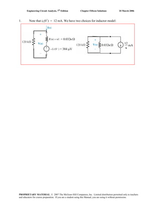
  • 1. Engineering Circuit Analysis, 7th Edition 1. Chapter Fifteen Solutions 10 March 2006 Note that iL(0+) = 12 mA. We have two choices for inductor model: = 0.032s Ω 0.032s Ω = 384 μV 12 mA s PROPRIETARY MATERIAL. © 2007 The McGraw-Hill Companies, Inc. Limited distribution permitted only to teachers and educators for course preparation. If you are a student using this Manual, you are using it without permission.
  • 2. Engineering Circuit Analysis, 7th Edition 2. Chapter Fifteen Solutions 10 March 2006 iL(0-) = 0, vC(0+) = 7.2 V (‘+’ reference on left). There are two possible circuits, since the inductor is modeled simply as an impedance: 1 Ω 0.002s 73 Ω 1 Ω 0.002s 7.2 V s 0.03s Ω 73 Ω + V(s) - 14.4 mA 0.03s Ω + V(s) - PROPRIETARY MATERIAL. © 2007 The McGraw-Hill Companies, Inc. Limited distribution permitted only to teachers and educators for course preparation. If you are a student using this Manual, you are using it without permission.
  • 3. Engineering Circuit Analysis, 7th Edition Chapter Fifteen Solutions 10 March 2006 3. (a) Z m (s) = 2s 2000 / s 20s 1000 + = + 20 + 0.1s 2 + 1000 / s s + 200 s + 500 20s 2 + 10, 000s + 1000s + 200, 000 = = s 2 + 700s + 100, 000 (b) Zin(-80) = - 10.95 Ω (c) Zin ( j80) = (d) YRL = 1 10 s + 200 + = 20 s 20s (e) YRC = 20s 2 + 11, 000s + 200, 000 s 2 + 700s + 100, 000 1 s + 500 + 0.001s = 2 1000 (f) −128, 000 + j880, 000 + 200, 000 = 8.095∠54.43° Ω −6400 + j 56, 000 + 100, 000 s + 200 + 0.5 + 0.001s YRL + YRC s + 200 + 10s + 0.02s 2 = 20s = (s + 200) YRL YRC 0.001s 2 + 0.7s + 100 (0.001s + 0.5) 20s 20s 2 + 11, 000s + 200, 000 = = Z(s) s 2 + 700s + 100, 000 PROPRIETARY MATERIAL. © 2007 The McGraw-Hill Companies, Inc. Limited distribution permitted only to teachers and educators for course preparation. If you are a student using this Manual, you are using it without permission.
  • 4. Engineering Circuit Analysis, 7th Edition Chapter Fifteen Solutions 10 March 2006 4. 1 2 × 10⁻³ s 1 2 × 10⁻³ s 1 1 ⎛ ⎞ ⎛ ⎞ Zin = ⎜ 20 + = (20 + 500s-1) || (40 + 500s-1) || ⎜ 40 + −3 ⎟ −3 ⎟ 2 × 10 s ⎠ ⎝ 2 × 10 s ⎠ ⎝ = 80s 2 + 3000s +25000 6s 2 + 100s PROPRIETARY MATERIAL. © 2007 The McGraw-Hill Companies, Inc. Limited distribution permitted only to teachers and educators for course preparation. If you are a student using this Manual, you are using it without permission.
  • 5. Engineering Circuit Analysis, 7th Edition Zin = Zin ( j8) = (c) Zin (−2 + j 6) = (d) (e) 10 March 2006 50 16(0.2s) 50 16s 16s 2 + 50s + 4000 + = + = s 16 + 0.2s s s + 80 s 2 + 80s (a) (b) 5. Chapter Fifteen Solutions −1024 + 4000 + j 400 = 0.15842 − j 4.666 Ω −64 + j 640 16(4 − 36 − j 24) − 100 + j 300 + 4000 = 6.850∠ − 114.3° Ω −32 − j 24 − 160 + j 480 0.2 sR 50 0.2Rs 2 + 10s + 50R , + = s R + 0.2s 0.2s 2 + Rs 5R − 50 + 50 R Zin (−5) = ∴ 55R = 50, R = 0.9091 Ω 5 − 5R Zin = R = 1Ω PROPRIETARY MATERIAL. © 2007 The McGraw-Hill Companies, Inc. Limited distribution permitted only to teachers and educators for course preparation. If you are a student using this Manual, you are using it without permission.
  • 6. Engineering Circuit Analysis, 7th Edition 6. 2 mF → Chapter Fifteen Solutions 10 March 2006 1 Ω, 1 mH → 0.001s Ω, 2 × 10⁻³ s Zin = (55 + 500/ s) || (100 + s/ 1000) = s ⎞ 500 ⎞ ⎛ ⎛ ⎟ ⎜ 55 + ⎟ ⎜100 + 55s 2 + 5.5005 × 10⁶ s + 5 × 10⁷ s ⎠ ⎝ 1000 ⎠ ⎝ = s 500 s 2 + 5 × 10⁵ s + 1.55 × 10⁵ 155 + + s 1000 PROPRIETARY MATERIAL. © 2007 The McGraw-Hill Companies, Inc. Limited distribution permitted only to teachers and educators for course preparation. If you are a student using this Manual, you are using it without permission.
  • 7. Engineering Circuit Analysis, 7th Edition 7. Chapter Fifteen Solutions 10 March 2006 We convert the circuit to the s-domain: 1/sCμ Ω Vπ 1/sCπ Ω Vπ rπ R B and rπ + R B + rπ R BCπ s ZL = RC || RL = RCRL/ (RC + RL), we next connect a 1-A source to the input and write two nodal equations: Defining Zπ = RB || rπ || (1/sCπ) = 1 Solving, Vπ = = Vπ/ Zπ + (Vπ – VL)Cμ s -gmVπ = VL/ ZL + (VL – Vπ)Cμ s [1] [2] rπ R B (1 + Z L C μ s ) Z L rπ R BCπ C μ s 2 + (g m Z L rπ R BC μ + rπ R BCπ + rπ R BC μ + Z L rπ C μ +Z L R BC μ )s + rπ + R B Since we used a 1-A ‘test’ source, this is the input impedance. Setting both capacitors to zero results in rπ || RB as expected. PROPRIETARY MATERIAL. © 2007 The McGraw-Hill Companies, Inc. Limited distribution permitted only to teachers and educators for course preparation. If you are a student using this Manual, you are using it without permission.
  • 8. Engineering Circuit Analysis, 7th Edition 8. 0.115s Ω Chapter Fifteen Solutions 10 March 2006 460 μV I 2 s V 2 + 460 × 10−6 2.162 9400 s + = V(s) = 4700 0.115s + 4700 s (0.115s + 4700) 4700 + 0.115s = 18.8 81740 18.8 a b + = + + s + 40870 s (s + 40870) s + 40870 s s + 40870 where a = Thus, V(s) = 81740 s + 40870 = 2 and b = s =0 81740 s = -2 s = -40870 18.8 2 2 . Taking the inverse transform of each term, + s + 40870 s s + 40870 v(t) = [16.8 e-40870t + 2] u(t) V PROPRIETARY MATERIAL. © 2007 The McGraw-Hill Companies, Inc. Limited distribution permitted only to teachers and educators for course preparation. If you are a student using this Manual, you are using it without permission.
  • 9. Engineering Circuit Analysis, 7th Edition 9. Chapter Fifteen Solutions 10 March 2006 v(0-) = 4 V 303030 Ω s 9 s 4 V s I(s) 9 4 − 5 4.545 × 10⁻⁶ s s = = I(s) = 303030 s +0.2755 1.1 × 10⁶ + 303030 + 1.1 × 10⁶ s Taking the inverse transform, we find that i(t) = 4.545 e-0.2755t u(t) μA PROPRIETARY MATERIAL. © 2007 The McGraw-Hill Companies, Inc. Limited distribution permitted only to teachers and educators for course preparation. If you are a student using this Manual, you are using it without permission.
  • 10. Engineering Circuit Analysis, 7th Edition 10. Chapter Fifteen Solutions 10 March 2006 From the information provided, we assume no initial energy stored in the inductor. (a) Replace the 100 mH inductor with a 0.1s-Ω impedance, and the current source with a 25 × 10−6 A source. s 0.1s Ω 25 s V 25 × 10−6 ⎡ 2 (0.1s) ⎤ 5 × 10⁻⁶ 5 × 10-5 = = V ⎢ 2 + 0.1s ⎥ 0.1s + 2 s s + 20 ⎣ ⎦ Taking the inverse transform, (b) V(s) = v(t) = 50 e-20t mV The power absorbed in the resistor R is then p(t) = 0.5 v2(t) = 1.25 e-40t nW PROPRIETARY MATERIAL. © 2007 The McGraw-Hill Companies, Inc. Limited distribution permitted only to teachers and educators for course preparation. If you are a student using this Manual, you are using it without permission.
  • 11. Engineering Circuit Analysis, 7th Edition 11. Chapter Fifteen Solutions 10 March 2006 We transform the circuit into the s-domain, noting the initial condition of the capacitor: V1 V2 4/s Ω 2/s 6/s 2/s V Writing our nodal equations, V1 − 2 s + V1 − V2 + 1 1 2 V1 + 2 4 s =0 [1] s V2 − V1 V2 + =6 1 1 2 [2] We may solve to obtain V1 = and V1 = Taking the inverse transforms, and −6 ( s − 12 ) s ( 3s + 20 ) 2 ( s + 44 ) s ( 3s + 20 ) = 3.6 −5.6 + s + 6.67 s = −3.73 4.4 + s + 6.67 s v1(t) = –5.6e–6.67t + 3.6 V, t ≥ 0 v2(t) = –3.73e–6.67t + 4.4 V, t ≥ 0 PROPRIETARY MATERIAL. © 2007 The McGraw-Hill Companies, Inc. Limited distribution permitted only to teachers and educators for course preparation. If you are a student using this Manual, you are using it without permission.
  • 12. Engineering Circuit Analysis, 7th Edition 12. Chapter Fifteen Solutions 10 March 2006 We transform the circuit into the s-domain, noting the initial condition of the inductor: V1 V2 (a) Writing our nodal equations, 4V1 − 3V2 = and −3V1 + 3V2 + 2 s [1] 2/s 4/s A 36 V V2 + 36 4 = 9s s or 9s Ω [2] 1⎞ ⎛ −3V1 + ⎜ 3 + ⎟ V2 = 0 9s ⎠ ⎝ We may solve to obtain and ⎛ ⎞ ⎜ 1 ⎟ 1 ⎛1⎞ 3 V1 = = ⎜ ⎟+ ⎜ ⎟ s ( 27s + 4 ) 2 ⎜ s + 4 ⎟ 2 ⎝ s ⎠ 27 ⎠ ⎝ 54 2 = V2 = 27s + 4 s + 4 27 Taking the inverse transforms, and 2 ( 27s + 1) v1(t) = 1.5–0.1481t + 0.5 V, t ≥ 0 v2(t) = 2e–0.1481t V, t ≥ 0 (b) PROPRIETARY MATERIAL. © 2007 The McGraw-Hill Companies, Inc. Limited distribution permitted only to teachers and educators for course preparation. If you are a student using this Manual, you are using it without permission.
  • 13. Engineering Circuit Analysis, 7th Edition 13. Chapter Fifteen Solutions 10 March 2006 (a) We transform the circuit into the s-domain, noting the initial condition of the capacitor: 1/s Ω 12/s I2 I1 9/s V Writing the two required mesh equations: 1⎞ 1 3 ⎛ ⎜ 6 + ⎟ I1 − I 2 = s⎠ s s ⎝ 1 1⎞ 9 ⎛ − I1 + ⎜12 + ⎟ I 2 = s s⎠ s ⎝ [1] [2] ⎛ ⎞ 2 ⎡ ( 3s + 1) ⎤ 2 1 ⎜ 1 ⎟ Solving yields I1 = ⎢ ⎥= − 3 ⎢ s ( 4s + 1) ⎥ 3s 6 ⎜ s + 1 ⎟ ⎣ ⎦ 4⎠ ⎝ 1 ⎡ ( 9s + 2 ) ⎤ 2 1 ⎛ 1 ⎞ ⎟ and I 2 = ⎢ ⎥= + ⎜ 3 ⎢ s ( 4s + 1) ⎥ 3s 12 ⎜ s + 1 ⎟ ⎣ ⎦ 4⎠ ⎝ Thus, taking the inverse Laplace transform, we obtain i1 (t ) = 2 1 −t4 − e A, t ≥ 0 3 6 and i2 (t ) = 2 1 − t4 + e A, t ≥ 0 3 12 (b) PROPRIETARY MATERIAL. © 2007 The McGraw-Hill Companies, Inc. Limited distribution permitted only to teachers and educators for course preparation. If you are a student using this Manual, you are using it without permission.
  • 14. Engineering Circuit Analysis, 7th Edition 14. Chapter Fifteen Solutions 10 March 2006 (a) We transform the circuit into the s-domain, noting the initial condition of the inductor: I1 9/s sΩ I2 8V Writing the two required mesh equations: 9 +8 s −sI1 + (10 + s ) I 2 = −8 ( 2 + s ) I1 − sI 2 = [1] [2] ⎡ ⎤ 1 ⎢ ( 89s + 90 ) ⎥ 35 ⎛ 1 ⎞ 4.5 ⎟+ Solving yields I1 = = ⎜ 12 ⎢ s s + 5 ⎥ 12 ⎜ s + 5 ⎟ s 3⎠ ⎢ ⎝ 3 ⎥ ⎣ ⎦ ⎡ ⎤ ⎛ ⎞ −7 ⎢ 1 ⎥=− 7 ⎜ 1 ⎟ and I 2 = 12 ⎢ s + 5 ⎥ 12 ⎜ s + 5 ⎟ 3⎠ ⎢ ⎝ 3 ⎥ ⎣ ⎦ ( ( ) ) Thus, taking the inverse Laplace transform, we obtain i1 (t ) = 35 −1.667 t e + 4.5 A, t ≥ 0 12 and i2 (t ) = − 7 −1.667 t A, t ≥ 0 e 12 (b) PROPRIETARY MATERIAL. © 2007 The McGraw-Hill Companies, Inc. Limited distribution permitted only to teachers and educators for course preparation. If you are a student using this Manual, you are using it without permission.
  • 15. Engineering Circuit Analysis, 7th Edition 15. Chapter Fifteen Solutions 10 March 2006 v(t) = 10e-2t cos (10t + 30o) V scos30o -10sin30o 0.866s - 5 cos (10t + 30 ) ⇔ = 2 2 s +100 s + 100 -at L {f(t)e } ⇔ F(s + a), so o V(s) = 10 0.866 ( s + 2 ) - 5 (s + 2) 2 + 100 = 8.66s - 16.34 s + 100 The voltage across the 5-Ω resistor may be found by simple voltage division. We first 50 Ω. Thus, note that Zeff = (10/s) || 5 = 5s + 10 ⎛ 50 ⎞ ⎜ ⎟ Vs 50 Vs 50 Vs ⎝ 5s + 10 ⎠ = = V5Ω = 2 ⎛ 50 ⎞ ( 0.5s + 5) ( 5s + 10 ) + 50 2.5s + 30s + 100 0.5s + 5 + ⎜ ⎟ ⎝ 5s + 10 ⎠ V 0.866s - 3.268 34.64s - 130.7 = (a) Ix = eff = 40 2 2 5 ⎡( s + 2 ) + 100 ⎤ ⎡s 2 + 12s + 40 ⎤ ⎡( s + 2 ) + 100 ⎤ ⎡( s + 6 )2 + 100 ⎤ ⎣ ⎦ ⎣ ⎦ ⎦ ⎣ ⎦⎣ (b) Taking the inverse transform using MATLAB, we find that ix(t) = e-6t [0.0915cos 2t - 1.5245 sin 2t] - e-2t [0.0915 cos10t - 0.3415 sin 10t] A PROPRIETARY MATERIAL. © 2007 The McGraw-Hill Companies, Inc. Limited distribution permitted only to teachers and educators for course preparation. If you are a student using this Manual, you are using it without permission.
  • 16. Engineering Circuit Analysis, 7th Edition 16. VC1 10 March 2006 2 Ω V2 s V1 3 s Chapter Fifteen Solutions 5 Ω s 8s Ω 5 V s Node 1: 0 = 0.2 (V1 – 3/ s) + 0.2 V1 s + 0.5 (V1 – V2) s Node 2: 0 = 0.5 (V2 – V1) s + 0.125 V2 s + 0.1 (V2 + 5/ s) Rewriting, (3.5 s 2 + s) V1 + 2.5 s 2 V2 = 3 -4 s 2 V1 + (4 s 2 + 0.8 s + 1) V2 = -4 [1] [2] Solving using MATLAB or substitution, we find that −20s 2 + 16s + 20 40s 4 + 68s3 + 43s 2 + 10s −20s 2 + 16s + 20 ⎛ 1 ⎞ = ⎜ ⎟ ⎝ 40 ⎠ s ( s + 0.5457 - j 0.3361)( s + 0.5457 + j 0.3361)( s + 0.6086 ) V1 (s) = which can be expanded: a b b* c V1 (s) = + + + s s + 0.5457 - j 0.3361 s + 0.5457 + j 0.3361 s + 0.6086 Using the method of residues, we find that a = 2, b = 2.511 ∠101.5o, b* = 2.511∠-101.5o and c = -1.003. Thus,taking the inverse transform, v1(t) = [2 – 1.003 e-0.6086t + 5.022 e-0.5457t cos (0.3361t – 101.5o)] u(t) V PROPRIETARY MATERIAL. © 2007 The McGraw-Hill Companies, Inc. Limited distribution permitted only to teachers and educators for course preparation. If you are a student using this Manual, you are using it without permission.
  • 17. Engineering Circuit Analysis, 7th Edition 17. Chapter Fifteen Solutions 10 March 2006 With zero initial energy, we may draw the following circuit: 2 s-1 Ω 3 V s 5 s-1 Ω 8sΩ 5 V s Define three clockwise mesh currents I1, I2, and I3 in the left, centre and right meshes, respectively. Mesh 1: -3/s + 5I1 + (5/s)I1 – (5/s)I2 = 0 Mesh 2: -(5/s)I1 + (8s + 7/s)I2 – 8s I3 = 0 Mesh 3: -8sI2 + (8s + 10)I3 – 5/s = 0 Rewriting, (5s + 5) I1 – 5 I2 -5 I1 + (8s2 +7) I2 – 8s2 I3 - 8s2 I2 + (8s2 + 10s) I3 = 3 = 0 = 5 [1] [2] [3] Solving, we find that I2(s) = = 2 20s + 32s + 15 20s 2 + 32s + 15 =⎛ 1 ⎞ ⎜ ⎟ 2 40s + 68s + 43s + 10 ⎝ 40 ⎠ ( s + 0.6086 )( s + 0.5457 - j 0.3361)( s + 0.5457 + j 0.3361) 3 a b b* + + ( s + 0.6086 ) ( s + 0.5457 - j 0.3361) ( s + 0.5457 + j 0.3361) where a = 0.6269, b = 0.3953∠-99.25o, and b* = 0.3955∠+99.25o Taking the inverse tranform, we find that o o i2(t) = [0.6271e-0.6086t + 0.3953e-j99.25 e(-0.5457 + j0.3361)t + 0.3953ej99.25 e(-0.5457 - j0.3361)t ]u(t) = [0.6271e-0.6086t + 0.7906 e-0.5457t cos(0.3361t + 99.25o)] u(t) PROPRIETARY MATERIAL. © 2007 The McGraw-Hill Companies, Inc. Limited distribution permitted only to teachers and educators for course preparation. If you are a student using this Manual, you are using it without permission.
  • 18. Engineering Circuit Analysis, 7th Edition 18. Chapter Fifteen Solutions 10 March 2006 We choose to represent the initial energy stored in the capacitor with a current source: V1 3 V s 5 Ω s • 2 Ω s ↑ 1.8 A V2 5 V s 8s Ω • Node 1: Node 2: Rewriting, 3 s + s V + s (V - V ) 1.8 = 1 1 2 5 5 2 5 V2 + 1 s s 0 = (V2 - V1 ) + V2 + 2 8s 10 V1 - (5s2 + 4s) V1 – 5s2 V2 = 18s + 6 -4s2 V1 + (4s2 + 0.8s + 1)V2 = -4 Solving, we find that V1(s) = [1] [2] 360s3 + 92s 2 + 114s + 30 s(40s3 + 68s 2 + 43s + 10) a b c c* + + + = s s + 0.6086 s + 0.5457 - j 0.3361 s + 0.5457 + j 0.3361 where a = 3, b = 30.37, c = 16.84 ∠136.3o and c* = 16.84 ∠-136.3o Taking the inverse transform, we find that o v1(t) = [3 + 30.37e-0.6086t + 16.84 ej136.3 e-0.5457t ej0.3361t o + 16.84 e-j136.3 e-0.5457t e-j0.3361t ]u(t) V = [3 + 30.37e-0.6086t + 33.68e-0.5457t cos (0.3361t + 136.3o]u(t) V PROPRIETARY MATERIAL. © 2007 The McGraw-Hill Companies, Inc. Limited distribution permitted only to teachers and educators for course preparation. If you are a student using this Manual, you are using it without permission.
  • 19. Engineering Circuit Analysis, 7th Edition 19. Chapter Fifteen Solutions 10 March 2006 We begin by assuming no initial energy in the circuit and transforming to the s-domain: V1 20 10 Ω s 2s Ω s+3 A (s + 3) 2 + 16 (a) via nodal analysis, we write: V 20s + 60 s = ( V1 - Vx ) + 1 2 (s + 3) + 16 10 5 V 120 s = x + ( Vx − V1 ) 2 (s + 3) + 16 2s 10 Vx 30 4 A (s + 3)2 + 16 [1] and [2] Collecting terms and solving for Vx(s), we find that Vx(s) = = 200s(s 2 + 9s + 12) 2s 4 + 17s3 + 90s 2 + 185s + 250 200s(s 2 + 9s + 12) ( s + 3 - j 4 )( s + 3 + j 4 )( s + 1.25 - j1.854 )( s + 1.25 + j1.854 ) (b) Using the method of residues, this function may be rewritten as a a* b b* + + + ( s + 3 - j 4 ) ( s + 3 + j 4 ) ( s + 1.25 - j1.854 ) ( s + 1.25 + j1.854 ) with a = 92.57 ∠ -47.58o, a* = 92.57 ∠ 47.58o, b = 43.14 ∠106.8o, b* = 43.14 ∠-106.8o Taking the inverse transform, then, yields o o vx(t) = [92.57 e-j47.58 e-3t ej4t + 92.57 ej47.58 e-3t e-j4t o o + 43.14ej106.8 e-1.25t ej1.854t + 43.14e-j106.8 e-1.25t e-j1.854t] u(t) = [185.1 e-3t cos (4t - 47.58o) + 86.28 e-1.25t cos (1.854t + 106.8o)] u(t) PROPRIETARY MATERIAL. © 2007 The McGraw-Hill Companies, Inc. Limited distribution permitted only to teachers and educators for course preparation. If you are a student using this Manual, you are using it without permission.
  • 20. Engineering Circuit Analysis, 7th Edition 20. Chapter Fifteen Solutions 10 March 2006 We model the initial energy in the capacitor as a 75-μA independent current source: 0.005s Ω 162.6s V s 2 + 4π 2 106 Ω s First, define Zeff = 106/s || 0.005s || 20 = ↑ V 75 μA s Ω 10 s + 0.005s + 200 -6 2 Then, writing a single KCL equation, 75 ×10-6 = V (s) 1 ⎛ 162.6s ⎞ + ⎜ V (s) - 2 ⎟ Zeff 20 ⎝ s + 4π 2 ⎠ which may be solved for V(s): V(s) = = 75s ( s 2 + 1.084 × 10⁵s + 39.48 ) s 4 + 5.5 × 10⁴s3 + 2 × 10⁸s 2 + 2.171× 10⁶s + 7.896 × 10⁹ 75s s 2 + 1.084 ×10⁵s + 12.57 ( ) ( s + 51085)( s + 3915)( s - j 6.283)( s + j 6.283) (NOTE: factored with higher-precision denominator coefficients using MATLAB to obtain accurate complex poles: otherwise, numerical error led to an exponentially growing pole i.e. real part of the pole was positive) a b c c* = + + + ( s + 51085 ) ( s + 3915 ) ( s - j 2π ) ( s + j 2π ) where a = -91.13, b = 166.1, c = 0.1277∠89.91o and c* = 0.1277∠-89.91o. Thus, consolidating the complex exponential terms (the imaginary components cancel), v(t) = [-91.13e-51085t + 166.1e-3915t + 0.2554 cos (2πt + 89.91o)] u(t) V (b) The steady-state voltage across the capacitor is V = [255.4 cos(2πt + 89.91o)] mV This can be written in phasor notation as 0.2554 ∠89.91o V. The impedance across which this appears is Zeff = [jωC + 1/jωL + 1/20]-1 = 0.03142 ∠89.91o Ω, so Isource = V/ Zeff = 8.129∠-89.91o A. Thus, isource = 8.129 cos 2πt A. (c) By phasor analysis, we can use simple voltage division to find the voltage division to find the capacitor voltage: (162.6∠0 ) ( 0.03142∠89.91o ) VC(jω) = = 0.2554∠89.92o V which agrees with 20 + 0.03142∠89.91o our answer to (a), assuming steady state. Dividing by 0.03142 ∠89.91o Ω, we find isource = 8.129 cos 2πt A. PROPRIETARY MATERIAL. © 2007 The McGraw-Hill Companies, Inc. Limited distribution permitted only to teachers and educators for course preparation. If you are a student using this Manual, you are using it without permission.
  • 21. Engineering Circuit Analysis, 7th Edition 21. Chapter Fifteen Solutions 10 March 2006 Only the inductor appears to have initial energy, so we model that with a voltage source: I1 I2 I4 0.001s Ω 1 mV 5.846s + 2.699 V s2 + 4 1333/s Ω 1000/s Ω I1 I3 6s V s +4 2 5.846s + 2.699 1333 ⎞ 1333 ⎛ = ⎜2 + I 2 - 2I 3 ⎟ I1 2 s +4 s ⎠ s ⎝ 0 = 0.005I1 – 0.001 + (0.001s + 1333/s) I2 – (1333/s)I1 – 0.001sI4 6s 0 = (2 + 1000/s)I3 – 2I1 – (1000/s)I4 + 2 s +4 0 = (0.001s + 1000/s) I4 - 0.001sI2 – (1000/s)I3 + 0.001 Mesh 1: Mesh 2: Mesh 3: Mesh 4: 154s − 2699 and s2 + 4 154s 4 - 7.378 × 10⁷ s3 - 1.912 × 10¹⁰s 2 - 4.07 × 10¹³s + 7.196 × 10¹⁴ I2 = 0.001 2333s 4 + 6.665 × 10⁵s3 + 1.333 × 10⁹s 2 + 5.332 × 10⁹ 0.4328∠ − 166.6o 0.4328∠ + 166.6o = + s + 142.8 + j 742 s + 142.8 - j 742 Solving, we find that I1 = −0.2 135.9∠ − 96.51o 135.9∠ + 96.51o + + 6.6 ×10⁻⁵ s - j2 s + j2 Taking the inverse transform of each, + i1(t) = 271.7 cos (2t – 96.51o) A and i2(t) = 0.8656 e-142.8t cos (742.3t + 166.6o) + 271.8 cos (2t – 96.51o) + 6.6×10⁻⁵ δ(t) A Verifying via phasor analysis, we again write four mesh equations: 6∠-13o = (2 – j666.7)I1 + j667I2 – 2I3 0 = (0.005 + j666.7)I1 + (j2x10-3 – j666.7)I2 – j2×10-3I4 -6∠0 = -2I1 + (2 – j500)I3 + j500I4 0 = -j2×10-3I2 + j500I3 + (j2×10-3 – j500)I4 Solving, we find I1 = 271.7∠-96.5o A and I2 = 272∠-96.5o A. From the Laplace analysis, we see that this agrees with our expression for i1(t), and as t → ∞, our expression for i2(t) → 272 cos (2t – 96.5o) in agreement with the phasor analysis. PROPRIETARY MATERIAL. © 2007 The McGraw-Hill Companies, Inc. Limited distribution permitted only to teachers and educators for course preparation. If you are a student using this Manual, you are using it without permission.
  • 22. Engineering Circuit Analysis, 7th Edition 22. Chapter Fifteen Solutions 10 March 2006 With no initial energy storage, we simply convert the circuit to the s-domain: V2 I2 V2 1667/s Ω s -2 I1 2000/s Ω V2 I3 0.002s Ω Writing a supermesh equation, 1 1 2000 2000 = 100I1 + I1 + I 3 + 0.002sI 3 I2 2 −4 6 × 10 s s s s we next note that I2 = -5V2 = -5(0.002s)I3 = -0.01sI3 and I3 – I1 = 3V2 = 0.006sI3, or I1 = (1 – 0.006s)I3, we may write I3 = 1 −0.598s + 110s 2 + 3666s 3 1 −0.0012s + 0.22s3 + 7.332s 2 7.645 ×10⁻⁵ 4.167 × 10⁻³ 4.091×10⁻³ 0.1364 − + =− + s − 212.8 s + 28.82 s s2 Taking the inverse transform, v2(t) = -7.645×10⁻⁵ e212.8t + 4.167×10⁻³ e-28.82t – 4.091×10⁻³ + 0.1364 t] u(t) V V2(s) = I3/ 0.002s = (a) v2(1 ms) = (b) v2(100 ms) = (c) v2(10 s) = 4 -5.58×10⁻⁷ V -1.334×10⁵ V -1.154×10920 V. This is pretty big- best to start running. PROPRIETARY MATERIAL. © 2007 The McGraw-Hill Companies, Inc. Limited distribution permitted only to teachers and educators for course preparation. If you are a student using this Manual, you are using it without permission.
  • 23. Engineering Circuit Analysis, 7th Edition 23. Chapter Fifteen Solutions 10 March 2006 We need to write three mesh equations: Mesh 1: 5.846s + 2.699 1333 ⎞ ⎛ = ⎜2 + ⎟ I1 - 2I 3 2 s +4 s ⎠ ⎝ Mesh 3: 0 = (2 + 1000/s)I3 – 2I1 – (1000/s)I4 + 6s s +4 0 = (0.001s + 1000/s) I4 – (1000/s)I3 + 10-6 Mesh 4: Solving, I1 = −0.001s (154s 3 2 - 2.925 ×10⁶s 2 + 1.527 × 10⁸s - 2.699 × 10⁹ ) 2333s 4 + 6.665 ×10⁵s3 + 1.333 × 10⁹s 2 + 2.666 × 10⁶s + 5.332 × 10⁹ 0.6507∠12.54o 0.6507∠ − 12.54o = + s + 142.8 − j 742.3 s + 142.8 + j 742.3 0.00101∠ − 6.538o 0.00101∠6.538o − 6.601× 10⁻⁵ + + s − j2 s + j2 which corresponds to i1(t) = 1.301 e-142.8t cos (742.3t + 12.54o) + 0.00202 cos (2t – 6.538o) – 6.601×10⁻⁵ δ(t) A and I3 = (154s −0.001 = 4 + 3.997 × 10⁶s3 + 1.547 × 10⁸s 2 + 3.996 × 10¹²s - 2.667 ×10⁶ (s 2 )( + 4 2333s + 6.665 ×10 s + 1.333 ×10 2 5 9 ) ) 0.7821∠ − 33.56o 0.7821∠33.56o + s + 142.8 − j 742.3 s + 142.8 + j 742.3 1.499∠179.9o 1.499∠ − 179.9o + s − j2 s + j2 which corresponds to i3(t) = 1.564 e-142.8t cos (742.3t – 33.56o) + 2.998 cos (2t + 179.9o) A + 2 The power absorbed by the 2-Ω resistor, then, is 2 ⎡i1 (t ) − i3 (t ) ⎤ or ⎣ ⎦ p(t) = 2[1.301 e-142.8t cos (742.3t + 12.54o) + 0.00202 cos (2t – 6.538o) – 6.601×10⁻⁵ δ(t) - 1.564 e-142.8t cos (742.3t – 33.56o) - 2.998 cos (2t + 179.9o)]2 W PROPRIETARY MATERIAL. © 2007 The McGraw-Hill Companies, Inc. Limited distribution permitted only to teachers and educators for course preparation. If you are a student using this Manual, you are using it without permission.
  • 24. Engineering Circuit Analysis, 7th Edition 24. Chapter Fifteen Solutions (a) We first define Zeff = RB || rπ || (1/sCπ) = 10 March 2006 rπ R B . Writing two nodal rπ + R B + rπ R B Cπ s equations, then, we obtain: and 0 = (Vπ – VS)/ RS + Vπ (rπ + RB + rπ RBCπs)/rπRB + (Vπ – Vo)Cμ s -gmVπ = Vo(RC + RL)/RCRL + (Vo – Vp) Cμ s Solving using MATLAB, we find that Vo = rπ R B R C R L (-g m + C μ s) [R s rπ R B R C R L Cπ C μ s 2 + (R s rπ R B R C Cπ + R s rπ R B R C C μ Vs + R s rπ R B R L Cπ + R s rπ R B R L C μ + rπ R B R C R L C μ + R s rπ R C R L C μ + R s R B R C R L C μ + g m R s rπ R B R C R L C μ )s + rπ R B R C + R s rπ R C + R s R B R C + rπ R B R L + R s rπ R L + R s R B R L ]−1 (b) Since we have only two energy storage elements in the circuit, the maximum number of poles would be two. The capacitors cannot be combined (either series or in parallel), so we expect a second-order denominator polynomial, which is what we found in part (a). PROPRIETARY MATERIAL. © 2007 The McGraw-Hill Companies, Inc. Limited distribution permitted only to teachers and educators for course preparation. If you are a student using this Manual, you are using it without permission.
  • 25. Engineering Circuit Analysis, 7th Edition Chapter Fifteen Solutions 10 March 2006 25. (a) IC I 500/s Ω 3/s 0.001s Ω (b) ZTH = (5 + 0.001s) || (500/ s) = VTH = (3/ s)ZTH 2500s + 0.5 Ω 0.001s 2 + 5s + 500 7.5 × 10⁶s + 1500 = V s s 2 + 5000s + 5 × 10⁵ ( ) 7.5 ×10⁶s + 1500 2500s + 0.5 ⎛ ⎞ s ( s 2 + 505000 ) ⎜1 + ⎟ 0.001s 2 + 5s + 500 ⎠ ⎝ 2.988 10.53∠-89.92o 10.53∠+89.92o =− + + s + 2.505 × 10⁶ s + j 710.6 s − j 710.6 (c) V1Ω = VTH 1 = 1 + Z TH + 2.956 2.967 × 10⁻³ + s + 0.1998 s 6 Thus, i1Ω = v1Ω(t) = [-2.988 e-2.505×10 t + 2.956 e-0.1998t + 2.967×10⁻³ + 21.06 cos(710.6t + 89.92o)] u(t) PROPRIETARY MATERIAL. © 2007 The McGraw-Hill Companies, Inc. Limited distribution permitted only to teachers and educators for course preparation. If you are a student using this Manual, you are using it without permission.
  • 26. Engineering Circuit Analysis, 7th Edition Chapter Fifteen Solutions 10 March 2006 26. (a) IC I 20/s ± 500/s Ω 0.001s Ω (b) ZTH = 0, VTH = 20/ s V so IN = ∞ ⎛ 20 ⎞ ⎜ ⎟ s (c) IC = ⎝ ⎠ = 0.04 A . Taking the inverse transform, we obtain a delta function: ⎛ 500 ⎞ ⎜ ⎟ ⎝ s ⎠ iC(t) = 40δ(t) mA. This “unphysical” solution arises from the circuit above attempting to force the voltage across the capacitor to change in zero time. PROPRIETARY MATERIAL. © 2007 The McGraw-Hill Companies, Inc. Limited distribution permitted only to teachers and educators for course preparation. If you are a student using this Manual, you are using it without permission.
  • 27. Engineering Circuit Analysis, 7th Edition Chapter Fifteen Solutions VTH ⎛ ⎛ 1⎞ ⎞⎛ 1 ⎞ ⎜ ⎜ 3 + s ⎟ ||10s ⎟ ⎜ ⎟ 70 ⎛7⎞ ⎠ ⎟⎜ s ⎟ = V = ⎜ ⎟⎜ ⎝ 2 ⎝ s ⎠ ⎜ 3 + ⎛ 3 + 1 ⎞ ||10s ⎟ ⎜ 3 + 1 ⎟ 60s + 19s + 3 ⎜ ⎟ ⎜ ⎟⎝ s⎠ s⎠ ⎝ ⎝ ⎠ ZTH 27. 10 March 2006 ⎛ 1 ⎞⎛ 9 + 60s ⎞ ⎜ ⎟⎜ ⎟ 30s ⎞ ⎝ s ⎠⎝ 3 + 10s ⎠ 9 + 60s ⎛1⎞ ⎛ Ω = ⎜ ⎟ || ⎜ 3 + = = ⎟ 1 9 + 60s 3 + 10s ⎠ 60s 2 + 19s + 3 ⎝s⎠ ⎝ + s 3 + 10s ZTotal = 9 + 60s 420s 4 + 133s3 + 21s 2 + 60s + 9 +7s 2 = Ω 60s 2 + 19s + 3 60s 2 + 19s + 3 Thus, ⎞ 70 60s 2 + 19s + 3 ⎛ ⎞⎛ I (s) = ⎜ ⎟A ⎟⎜ 2 4 3 2 ⎝ 60s + 19s + 3 ⎠ ⎝ 420s + 133s + 21s + 60s + 9 ⎠ 70 = A 4 3 420s + 133s + 21s 2 + 60s + 9 PROPRIETARY MATERIAL. © 2007 The McGraw-Hill Companies, Inc. Limited distribution permitted only to teachers and educators for course preparation. If you are a student using this Manual, you are using it without permission.
  • 28. Engineering Circuit Analysis, 7th Edition 28. Chapter Fifteen Solutions 10 March 2006 We begin by noting that the source is not really a dependent source – it’s value is not based on a voltage or current parameter. Therefore, we should treat it as an independent source. 2 (2s + 10) 2 2s + 10 s Zth = || (2s + 10) = Ω = 2 2 s + (2s + 10) s + 5s + 1 s 2 ⎛ ⎞ ⎜ ⎟ ⎡⎛ 9 ⎞ ⎤ 90 s V Vth = ⎜ ⎟ ⎢⎜ ⎟ (10) ⎥ = 2 2 ⎟ ⎣⎝ s ⎠ ⎦ s(s + 5s + 1) ⎜ 10 + 2s + s⎠ ⎝ PROPRIETARY MATERIAL. © 2007 The McGraw-Hill Companies, Inc. Limited distribution permitted only to teachers and educators for course preparation. If you are a student using this Manual, you are using it without permission.
  • 29. Engineering Circuit Analysis, 7th Edition 29. Chapter Fifteen Solutions 10 March 2006 Beginning with the source on the left (10/s V) we write two nodal equations: ′ V1′ − V2 s ⎛ ′ 10 ⎞ 1 V1′ + + = 0 ⎜ V1 ⎟ s ⎠ 47000 30303 56 + 336 × 10-6s ⎝ V2′ V2′ − V1′ s V2′ + + = 0 47000 10870 56 + 336 × 10-6s Solving, 303030(0.3197 ×10¹³ + 0.1645 ×10¹¹s + 98700s 2 ) ′= V1 s(0.4639 × 10¹⁰s3 + 0.7732 ×10¹⁵s 2 + 0.5691×10¹⁸s + 0.1936 ×10¹⁸ ) V2′ = 0.9676 ×10¹⁸ s(0.4639 ×10¹⁰s3 + 0.7732 ×10¹⁵s 2 + 0.5691×10¹⁸s + 0.1936 ×10¹⁸ ) Shorting out the left source and activating the right-hand source (5 – 3/s) V: V1′′ − V2′′ 1 s V1′′ + V1′′ + = 0 47000 30303 56 + 336 ×10-6s V2′′ - 5 + 47000 3 s + V2′′ − V1′′ s V2′′ + = 0 10870 56 + 336 ×10-6s Solving, V1′′ = 0.9676 ×10¹⁷ (5s − 3) s(0.4639 ×10¹⁰s3 + 0.7732 ×10¹⁵s 2 + 0.5691×10¹⁸s + 0.1936 ×10¹⁸ ) 7609(705000s3 + 0.1175 × 10¹²s 2 + 0.6359 × 10¹⁴s - 0.3819 ×10¹⁴ ) s(0.4639 × 10¹⁰s3 + 0.7732 ×10¹⁵s 2 + 0.5691×10¹⁸s + 0.1936 ×10¹⁸ ) Adding, we find that 30303(0.2239 ×10¹³ + 0.1613 ×10¹³s + 98700s 2 ) V1 = s(0.4639 ×10¹⁰s3 + 0.7732 ×10¹⁵s 2 + 0.5691×10¹⁸s + 0.1936 ×10¹⁸ ) V2′′ = V2 = 7609(705000s3 + 0.1175 ×10¹²s 2 + 0.6359 ×10¹⁴s + 0.8897 ×10¹⁴ ) s(0.4639 ×10¹⁰s3 + 0.7732 × 10¹⁵s 2 + 0.5691×10¹⁸s + 0.1936 ×10¹⁸ ) (b) Using the ilaplace() routine in MATLAB, we take the inverse transform of each: v1(t) = [3.504 + 0.3805×10⁻² e-165928t – 0.8618 e-739t – 2.646 e-0.3404t] u(t) V v2(t) = [3.496 – 0.1365×10⁻² e-165928t + 0.309 e-739t – 2.647 e-0.3404t] u(t) V PROPRIETARY MATERIAL. © 2007 The McGraw-Hill Companies, Inc. Limited distribution permitted only to teachers and educators for course preparation. If you are a student using this Manual, you are using it without permission.
  • 30. Engineering Circuit Analysis, 7th Edition 30. Chapter Fifteen Solutions 10 March 2006 (10/ s)(1/47000) = 2.128×10⁻⁴/ s A (5 – 3/s)/ 47000 = (1.064 – 0.6383/ s)×10-4 A 1.424 ×10⁹ Ω 47000s + 30303 5.109 ×10⁸ Ω ZR = 47000 || (10870/ s) = 47000s + 10870 ZL = 47000 || (30303/ s) = Convert these back to voltage sources, one on the left (VL) and one on the right (VR): ⎛ 1.424 ×10⁹ ⎞ 3.0303 × 10⁵ -4 VL = (2.128×10 / s ) ⎜ V ⎟ = ⎝ 47000s + 30303 ⎠ s ( 47000s + 30303) ⎛ 5.109 ×10⁸ ⎞ VR = (1.064 – 0.6383/ s)×10-4 ⎜ ⎟ ⎝ 47000s + 10870 ⎠ 54360 32611 = 47000s + 10870 s ( 47000s + 10870 ) Then, I56Ω = VL − VR Z L + Z R + 336 × 10-6s +56 = −6250 = 2.555 × 10⁹s 2 - 1.413 × 10¹⁰s - 4.282 × 10⁹ s 4.639 × 10⁹ s3 + 7.732 × 10¹⁴s 2 + 5.691× 10¹⁷s + 1.936 ×10¹⁷ ( ) −18 0.208 0.0210 1.533 × 10 − − 5 s + 1.659 ×10 s + 739 s + 0.6447 2.658 ×10⁻⁵ 2.755 × 10⁻¹⁸ 1.382 ×10⁻⁴ + + + s + 0.3404 s + 0.2313 s Thus, i56Ω(t) = [0.208 exp(-1.659×10⁵t) – 0.0210 exp(-739t) – 1.533×10⁻¹⁸ exp(-.06447t) + 2.658×10⁻⁵ exp(-0.3404t) + 2.755×10⁻¹⁸ exp(-0.2313t) + 1.382×10⁻⁴] u(t) A. The power absorbed in the 56-Ω resistor is simply 56 [i56Ω(t)]2 or 56 [0.208 exp(-1.659×10⁵t) – 0.0210 exp(-739t) – 1.533×10⁻¹⁸ exp(-.06447t) + 2.658×10⁻⁵ exp(-0.3404t) + 2.755×10⁻¹⁸ exp(-0.2313t) + 1.382×10⁻⁴]2 W PROPRIETARY MATERIAL. © 2007 The McGraw-Hill Companies, Inc. Limited distribution permitted only to teachers and educators for course preparation. If you are a student using this Manual, you are using it without permission.
  • 31. Engineering Circuit Analysis, 7th Edition 31. Chapter Fifteen Solutions 10 March 2006 (a) Begin by finding ZTH = ZN: ZTH = 47000 + (30303/ s) || [336×10-6 s + 56 + (10870/ s) || 47000] = 4.639 ×10⁹s3 + 7.732 ×10¹⁴s 2 + 5.691×10¹⁷s + 1.936 ×10¹⁷ Ω 98700s3 + 1.645 ×10¹⁰s 2 + 1.21×10¹³s + 2.059 ×10¹² To find the Norton source value, define three clockwise mesh currents I1, I2 and I3 in the left, centre and right hand meshes, such that IN(s) = -I1(s) and the 10/s source is replaced by a short circuit. (47000 + 30303/ s) I1 - (30303/ s) I2 (10870/ s + 56 + 336×10-6 s + 30303/ s) I2 - (30303/ s) I1 – (10870/ s)I3 (47000 + 10870/ s) I3 - (10870/ s)I2 = -5 + 3/ s Solving, 2.059 ×10¹² (5s - 3) IN = -I1 = s(4.639 ×10⁹s3 + 7.732 ×10¹⁴s 2 + 5.691×10¹⁷s + 1.936 ×10¹⁷ ) =0 =0 (b) Isource = (10/ s) (1/ ZTH) - IN(s) = 0.001(0.4579 × 10¹³s6 + 0.1526 ×10¹⁹s5 + 0.1283 ×10 24s 4 + 0.1792 × 1027s3 + 0.6306 × 1029s 2 + 0.3667 × 1029s + 0.5183 ×1028 )[s(4639s3 + 0.7732 ×10⁹s 2 + 0.5691×10¹²s + 0.1936 ×10¹² )(0.4639 ×10¹⁰s3 +0.7732 × 10¹⁵s 2 + 0.5691× 10¹⁸s + 0.1936 × 10¹⁸ )]-1 Taking the inverse transform using the MATLAB ilaplace() routine, we find that isource(t) = 0.1382×10⁻³ + 0.8607×10⁻⁸ exp(-165930t) + 0.8723×10⁻⁷exp(-739t) + 0.1063×10⁻³ exp(-0.3403t) – 0.8096×10⁻⁷ exp(-165930t) + 0.1820×10⁻⁴ exp(-739t) – 0.5×10⁻⁴ exp(-0.3404t) isource(1.5 ms) = 2.0055×10⁻⁴ A = 200.6 μA PROPRIETARY MATERIAL. © 2007 The McGraw-Hill Companies, Inc. Limited distribution permitted only to teachers and educators for course preparation. If you are a student using this Manual, you are using it without permission.
  • 32. Engineering Circuit Analysis, 7th Edition 32. Chapter Fifteen Solutions 10 March 2006 5s . s +4 (a) Define four clockwise mesh currents I1, I2, I3 and Ix in the top left, top right, bottom left and bottom right meshes, respectively. Then, We begin by shorting the 7 cos 4t source, and replacing the 5 cos 2t source with 5s s +4 0 0 0 V1′ 2 = (12 + 1/2s) I3 – 7 I1 – (1/ 2s) Ix [1] = = = = 2 [2] [3] [4] [5] -4 Ix + (9.5 + s) I1 – s I2 – 7 I3 (3 + s + 2/ s) I2 – s I1 – 3 Ix (4 + 3s + 1/2s) Ix – 3 I2 – (1/2s) I3 (I3 – Ix) (2s) Solving all five equations simultaneously using MATLAB, we find that V1′ = 20s3 (75s3 + 199s 2 + 187s + 152) 1212s6 + 3311s5 + 7875s 4 + 15780s3 + 12408s 2 + 10148s + 1200 7s . s + 16 Define four clockwise mesh currents I1, I2, I3 and Ix in the bottom left, top left, top right and bottom right meshes, respectively (note order changed from above). Then, Next we short the 5 cos 2t source, and replace the 7 cos 4t source with 0 = (12 + 1/2s) I1 – 7 I2 – (1/ 2s) Ix 0 = -4 Ix + (9.5 + s) I2 – s I3 – 7 I1 − 7s = (3 + s + 2/ s) I3 – s I2 – 3 Ix s + 16 0 = (4 + 3s + 1/2s) Ix – 3 I3 – (1/2s) I1 V1′′ = (I1 – Ix) (2s) 2 2 [1] [2] [3] [4] [5] Solving all five equations simultaneously using MATLAB, we find that V1′′ = -56s 4 (21s 2 - 8s - 111) 1212s 6 + 3311s5 + 22420s 4 + 55513s3 + 48730s 2 + 40590s + 4800 ( ) The next step is to form the sum V1(s) = V1′ + V1′′ , which is accomplished in MATLAB using the function symadd(): V1 = symadd(V1prime, V1doubleprime); V1(s) = ( 4s3 (81s5 + 1107s 4 + 7313s3 + 17130s 2 + 21180s + 12160) s 2 + 4 1212s 6 + 3311s5 + 22420s 4 + 55513s 3 + 48730s 2 + 40590s + 4800 )( ) (b) Using the ilaplace() routine from MATLAB, we find that v1(t) = [0.2673 δ(t) + 6.903×10⁻³ cos 2t – 2.403 sin 2t – 0.1167 e-1.971t – 0.1948 e-0.3315t cos 0.903t + 0.1611 e-0.3115t sin 0.903t – 0.823×10⁻³ e-0.1376t + 3.229 cos 4t + 3.626 sin 4t] u(t) V PROPRIETARY MATERIAL. © 2007 The McGraw-Hill Companies, Inc. Limited distribution permitted only to teachers and educators for course preparation. If you are a student using this Manual, you are using it without permission.
  • 33. Engineering Circuit Analysis, 7th Edition 33. Chapter Fifteen Solutions 10 March 2006 (a) We can combine the two sinusoidal sources in the time domain as they have the same frequency. Thus, there is really no need to invoke source transformation as such to find the current. 65 cos 103t ⇔ 65s , and 13 mH → 0.013s Ω s + 106 2 We may therefore write 1 5000s ⎛ 65s ⎞ ⎛ ⎞ I(s) = ⎜ 2 ⎟ = 2 6 ⎟⎜ ⎝ s + 10 ⎠ ⎝ 83 + 0.013s ⎠ ( s + 106 ) ( s + 6385 ) =− 0.7643 0.3869∠ − 8.907 o 0.3869∠8.907o + + ( s + 6385) s - j103 s + j103 ( ) ( ) (b) Taking the inverse transform, i(t) = [-0.7643 e-6385t + 0.7738 cos (103t – 8.907o)] u(t) A (c) The steady-state value of i(t) is simply 0.7738 cos (103t – 8.907o) A. PROPRIETARY MATERIAL. © 2007 The McGraw-Hill Companies, Inc. Limited distribution permitted only to teachers and educators for course preparation. If you are a student using this Manual, you are using it without permission.
  • 34. Engineering Circuit Analysis, 7th Edition 34. Chapter Fifteen Solutions 10 March 2006 (a) 7s 7 = 2 2 s 3s − 9s + 4 3 s − 3s + 4 ( Poles at ) ( 3 ) = 7 3 ⎛ 3 11 ⎞ ⎛ 3 11 ⎞ ⎟ ⎜s − + ⎟⎜s − − 12 ⎠ ⎝ 2 12 ⎠ ⎝ 2 3 11 ± , double zero at ∞ . 2 12 ( s + 1)( s − 1) s2 − 1 (b) 2 = ( s + 2s + 4 )( s2 + 1) s + 1 + j 3 s + 1 − j 3 ( s + j )(s − j ) ( )( ) Zeroes at s = –1, + 1, ∞ Poles at −1 + j 3, − 1 − j 3, ± j PROPRIETARY MATERIAL. © 2007 The McGraw-Hill Companies, Inc. Limited distribution permitted only to teachers and educators for course preparation. If you are a student using this Manual, you are using it without permission.
  • 35. Engineering Circuit Analysis, 7th Edition 35. Chapter Fifteen Solutions 10 March 2006 (a) 3s 2 3s = 2 s s + 4 ( s − 1) ( s + j 2 )( s − j 2 )( s − 1) ( ) Poles at ± j 2, 1 ; zeroes at s = 0, ∞ . s 2 + 2s − 1 = (b) 2 s 4s 2 + 2s + 1 s 2 − 1 ( )( ) (s + 1 + 2 )(s + 1 − 2 ) ⎛ 1 3 ⎞⎛ 1 3⎞ s2 ⎜ s + + j ⎟⎜ s + − j ⎟ ( s + 1)( s − 1) 4 4 ⎠⎝ 4 4 ⎠ ⎝ 1 3 Poles at s = ±1, − ± j , double at s = 0 4 4 Zeroes at −1 ± j 2, ∞ PROPRIETARY MATERIAL. © 2007 The McGraw-Hill Companies, Inc. Limited distribution permitted only to teachers and educators for course preparation. If you are a student using this Manual, you are using it without permission.
  • 36. Engineering Circuit Analysis, 7th Edition 36. (a) Chapter Fifteen Solutions 10 March 2006 5⎞ ⎛ ⎜ 5 + ⎟ (2 + 5s) (5s + 5)(2 + 5s) 25s 2 + 35s + 10 s⎠ Z in = ⎝ = = 5s + 7 + 5 / s 5s 2 + 7s + 5 5s 2 + 7s + 5 5s 2 + 7s + 5 ∴ Yin (s) = 25s 2 + 35s + 10 −1.4 ± 1.96 − 1.6 = −1, − 0.4s −1 2 −1.4 ± 1.96 − 4 Zeros: s 2 + 1.4s + 1 = 0, s = = −0.7 ± j 0.7141s −1 2 (b) Poles: s 2 + 1.4s + 0.2 = 0, s = (c) Poles: same; s = -1, -0.4 s-1 (d) Zeros: same; s = −0.7 ± j 0.7141 s −1 PROPRIETARY MATERIAL. © 2007 The McGraw-Hill Companies, Inc. Limited distribution permitted only to teachers and educators for course preparation. If you are a student using this Manual, you are using it without permission.
  • 37. Engineering Circuit Analysis, 7th Edition 37. Chapter Fifteen Solutions 10 March 2006 (a) Regarding the circuit of Fig. 15.45, we replace each 2-mF capacitor with a 500/ s Ω impedance. Then, 500 ⎞⎛ 500 ⎞ ⎛ ⎜ 20 + ⎟⎜ 40 + ⎟ (s + 25)(s + 12.5) s ⎠⎝ s ⎠ ⎝ Zin(s) = = 13.33 100 s(s + 1.667) 60 + s Reading from the transfer function, we have zeros at s = -25 and -12.5 s-1, and poles at s = 0 and s = -1.667 s-1. (b) Regarding the circuit of Fig. 15.47, we replace the 2-mF capacitor with a 500/ s Ω impedance and the 1-mH inductor with a 0.001s-Ω impedance. Then, 500 ⎞ ⎛ 500 (s + )(s + 105 ) ⎜ 55 + ⎟ (100 + 0.001s ) s ⎠ ⎝ 55 = 55 Zin(s) = 500 s + 1.55 ×10⁵ ) (s + 3.226) ( 155 + + 0.001s s Reading from the transfer function, we have zeros at s = -9.091 and -105 s-1, and 5 poles at s = -1.55×10 and s = -3.226 s-1. PROPRIETARY MATERIAL. © 2007 The McGraw-Hill Companies, Inc. Limited distribution permitted only to teachers and educators for course preparation. If you are a student using this Manual, you are using it without permission.
  • 38. Engineering Circuit Analysis, 7th Edition 38. Y(s) : zeros at s = 0; − 10; (a) Y (s) = Chapter Fifteen Solutions 10 March 2006 poles at s = −5, − 20 s −1 ; Y(s) → 12 S as s → ∞ Ks(s + 10) , K = 12 ∴ (s + 5)(s + 20) 12s(s + 10) 12s 2 + 120s = 2 (s + 5)(s + 20) s + 25s + 100 −1200 + j1200 ∴ Y ( j10) = = 4.800 + j 4.800 = 6.788∠45° S −100 + j 250 + 100 Y (s) = (b) Y ( − j10) = 6.788∠ − 45° S (c) Y(−15) = (d) 5 + Y (s) = 5 + 12(−15)(−5) = − 18 S (−10)5 −245 ± 2452 − 68(500) 12s 2 + 120s 17s 2 + 245s + 500 = ,s= (s + 5)(s + 20) 34 s 2 + 25s + 100 Zeros: s = −2.461 and − 11.951 s -1 ; Poles: s = −5, − 20 s -1 PROPRIETARY MATERIAL. © 2007 The McGraw-Hill Companies, Inc. Limited distribution permitted only to teachers and educators for course preparation. If you are a student using this Manual, you are using it without permission.
  • 39. Engineering Circuit Analysis, 7th Edition 39. Chapter Fifteen Solutions 10 March 2006 1 1 0.2(6s + 9) 5(s + 1)(s + 4) + = ∴ Zin = 4 + s 5 + 5s (4 + s)(1 + s) 6(s + 1.5) (a) Yin = (b) Poles: s = − 1.5, ∞; Zeros: s = -1, -4 s-1 PROPRIETARY MATERIAL. © 2007 The McGraw-Hill Companies, Inc. Limited distribution permitted only to teachers and educators for course preparation. If you are a student using this Manual, you are using it without permission.
  • 40. Engineering Circuit Analysis, 7th Edition 40. H(s) = Chapter Fifteen Solutions 10 March 2006 s+2 (s + 5)(s 2 + 6s + 25) (a) δ(t) ⇔ 1, so the output is s+2 (s + 5)(s 2 + 6s + 25) (b) e-4t u(t) ⇔ 1 / (s + 4), so the output is (c) 2 cos 15t u(t) ⇔ s+2 (s + 4)(s + 5)(s 2 + 6s + 25) 2s ( s + 2 ) 2s , so the output is 2 (s + 225)(s + 5)(s 2 + 6s + 25) s + 225 2 (d) t e-t u(t) ⇔ 1/ (s + 1), so the output is s+2 (s + 1)(s + 5)(s 2 + 6s + 25) (e) poles and zeros of each: (a): zero at s = -2, poles at s = -5, -3 ± j4 (b): zero at s = -2, poles at s = -4, -5, -3 ± j4 (c): zeros at s = 0, -2, poles at s = ± j15, -5, -3 ± j4 (d): zero at s = -2, poles at s = -1, -5, -3 ± j4 PROPRIETARY MATERIAL. © 2007 The McGraw-Hill Companies, Inc. Limited distribution permitted only to teachers and educators for course preparation. If you are a student using this Manual, you are using it without permission.
  • 41. Engineering Circuit Analysis, 7th Edition 41. h(t) = 5 [u(t) – u(t – 1)] sin πt y(t) = ∫ ∞ 0− Chapter Fifteen Solutions 10 March 2006 x(t) = 2[u(t) – u(t – 2)] h(λ ) x ( t − λ ) d λ t < 0: y(t) = 0 0 < t < 1: y(t) = 1 < t < 2: y(t) = 2 < t < 3: y(t) = t ∫ 10sin πλ d λ 0 1 ∫ 10sin πλ d λ 0 ∫ 1 t −2 = = 10 λ t cos πλ = 0 10 π (1 − cos π t ) 20 π 10sin πλ d λ = - 10 π 1 cos πλ = t −2 10 π [ −1 − cos(π t − 2π )] = (10/ π) (1 + cos πt) t > 3: y(t) = 0 PROPRIETARY MATERIAL. © 2007 The McGraw-Hill Companies, Inc. Limited distribution permitted only to teachers and educators for course preparation. If you are a student using this Manual, you are using it without permission.
  • 42. Engineering Circuit Analysis, 7th Edition 42. Chapter Fifteen Solutions 10 March 2006 f1(t) = e-5t u(t), f2(t) = (1 – e-2t) u(t) (a) f1 * f2 = ∫ ∞ 0- f1 ( λ ) f 2 ( t − λ ) d λ t < 0: f1 * f2 = 0 t > 0: f1 * f2 = ∫ t - 0 ( ) e −5λ 1 − e2λ − 2t d λ = 1 = − e−5λ 5 t 0 1 + e−2t e−3λ 3 t 0 ∫ (e t 0- −5 λ ) − e−2t e−3λ d λ 1 ⎛1 2 ⎞ = ⎜ + e−5t − e −2t ⎟ u (t ) 3 ⎝ 5 15 ⎠ (b) F1(s) = 1/ (s + 5), F2(s) = 1/s – 1/ (s + 2) 1 1 a b c − = + + F1(s) F2(s) = s ( s + 5) s s+2 s+5 ( s + 5)( s + 2 ) Where a = 0.2, b = -1/3, and c = -1/5 + 1/3 = 2/15. 1 ⎛1 2 ⎞ Taking the inverse transform, we find that f1 * f2 = ⎜ + e −5t − e −2t ⎟ u (t ) 3 ⎝ 5 15 ⎠ PROPRIETARY MATERIAL. © 2007 The McGraw-Hill Companies, Inc. Limited distribution permitted only to teachers and educators for course preparation. If you are a student using this Manual, you are using it without permission.
  • 43. Engineering Circuit Analysis, 7th Edition 43. Chapter Fifteen Solutions 10 March 2006 The impulse response is vo(t) = 4u(t) – 4u(t – 2) V, so we know that h(t) = 4u(t) – 4u(t – 2). vi(t) = 2u(t - 1), and vo(t) = h(t) * vi(t). ∞ ∞ ∫ h(λ )v ( t − λ ) d λ = 8∫ [u(λ ) − u(λ − 2)] u ( t − λ − 1) d λ 8∫ [1 − u (λ − 2)] u ( t − λ − 1) d λ . [1] Thus, vo(t) = or vo(t) = i 0 ∞ 0 0 For λ > 2, this integral is zero. Also, the second step function results in a zero value for the integral except when t – λ – 1 > 0, or λ < t – 1. With a lower limit of λ = 0, this means that t > 1. When t > 3, however, we do not must be careful to constrain λ to less than 2, so we split the integration into two parts: 1 < t < 3: vo = t > 3: vo = ∫ 2 0 ∫ t −1 0 8 d λ = 8t − 8 V 8 d λ = 16 V vo (V) 16 and, of course, for t < 1, the output is zero. 1 3 t (s) PROPRIETARY MATERIAL. © 2007 The McGraw-Hill Companies, Inc. Limited distribution permitted only to teachers and educators for course preparation. If you are a student using this Manual, you are using it without permission.
  • 44. Engineering Circuit Analysis, 7th Edition 44. Chapter Fifteen Solutions 10 March 2006 h(t) = 2e-3t u(t), x(t) = u(t) – δ(t) (a) y(t) = ∫ ∞ 0− h(λ ) x(t − λ )d λ t < 0 : y (t ) = 0 t ⎡ 1 t t > 0 : y (t ) = 2 ∫ − e −3λ [1 − δ (t − λ ) ] d λ = 2 ⎢ - e −3λ u (t ) 0 ⎢ 3 0 ⎣ 2 ⎛2 8 ⎞ = (1 − e −3t )u (t ) − 2e−3t u (t ) = ⎜ − e−3t ⎟ u (t ) 3 ⎝3 3 ⎠ (b) H (s) = 2 s+3 thus, Y(s) = ⎤ - e−3t u (t ) ⎥ ⎥ ⎦ 1 -1 s 2 ⎛1⎞ 8⎛ 1 ⎞ = ⎜ ⎟ - ⎜ ⎟ 3⎝s⎠ 3⎝ s + 3⎠ X(s) = 2 (1 - s ) s ( s + 3) Taking the inverse transform, we find that y(t) = 2 8 −3 t u (t ) − e u (t ) 3 3 PROPRIETARY MATERIAL. © 2007 The McGraw-Hill Companies, Inc. Limited distribution permitted only to teachers and educators for course preparation. If you are a student using this Manual, you are using it without permission.
  • 45. Engineering Circuit Analysis, 7th Edition 45. Chapter Fifteen Solutions h(t) = 5 u(t) - 5 u(t – 2), so H(s) = 10 March 2006 5 - 5e-2s s (a) vin(t) = 3δ(t), so Vin(s) = 3 Vout(s) = Vin(s) H(s) = 15 - 15e-2s . vout(t) = L-1{Vout(s)} = 15 u(t) – 15 u(t - 2) s (b) vin(t) = 3u(t), so Vin(s) = 3 s ⎛ 3⎞⎛ 5 ⎞ 15 15 -2s Vout(s) = Vin(s) H(s) = ⎜ ⎟ ⎜ - 5e-2s ⎟ = 2 e . s ⎝ s ⎠⎝ s ⎠ s vout(t) = L-1{Vout(s)} = 15 t u(t) – 15 u2(t - 2) = 15 t u(t) – 15 u (t - 2) (c) vin(t) = 3u(t) – 3u(t – 2), so Vin(s) = 3 - 3e-2s s ⎛3 ⎞⎛ 5 ⎞ 15 30 -2s Vout(s) = Vin(s) H(s) = ⎜ - 3e -2s ⎟ ⎜ - 5e-2s ⎟ = 2 e + 15e −4s . s ⎝s ⎠⎝ s ⎠ s -1 2 2 vout(t) = L {Vout(s)} = 15 t u(t) – 30 u (t - 2) + 15 u (t – 4) = 15 t u(t) – 30 u (t - 2) + 15 u(t) (d) vin(t) = 3 cos 3t, so Vin(s) = 3s s +9 2 15 15s -2s - 2 e . s +9 s +9 vout(t) = L-1{Vout(s)} = 5 sin 3t u(t) – 15 cos [3(t – 2)] u(t - 2) Vout(s) = Vin(s) H(s) = 2 PROPRIETARY MATERIAL. © 2007 The McGraw-Hill Companies, Inc. Limited distribution permitted only to teachers and educators for course preparation. If you are a student using this Manual, you are using it without permission.
  • 46. Engineering Circuit Analysis, 7th Edition 46. Chapter Fifteen Solutions 10 March 2006 (a) Since vo(t) = vin(t), H(s) = 1. Thus, h(t) = δ(t). ∞ ∞ −∞ −∞ (b) vo (t ) = ∫ vin ( x)h(t − x)dx = ∫ vin ( x)δ (t − x)dx = vin (t ) = 8u (t ) V PROPRIETARY MATERIAL. © 2007 The McGraw-Hill Companies, Inc. Limited distribution permitted only to teachers and educators for course preparation. If you are a student using this Manual, you are using it without permission.
  • 47. Engineering Circuit Analysis, 7th Edition 47. Chapter Fifteen Solutions 10 March 2006 (a) Since vo(t) = vin(t), H(s) = 1. Thus, h(t) = δ(t). ∞ ∞ −∞ −∞ (b) vo (t ) = ∫ vin ( x)h(t − x)dx = ∫ vin ( x)δ (t − x)dx = vin (t ) = 8e−t u (t ) V PROPRIETARY MATERIAL. © 2007 The McGraw-Hill Companies, Inc. Limited distribution permitted only to teachers and educators for course preparation. If you are a student using this Manual, you are using it without permission.
  • 48. Engineering Circuit Analysis, 7th Edition Chapter Fifteen Solutions 10 March 2006 48. I in = Vin = Vin 10 20(20 + 10 / s) + s 40 + 10 / s 10 10 ⎞ ⎛ + 20 20 ⎜ 20 + ⎟ s s ⎠ ⎝ Vin Vin 40s 2 + s = = = Vin 10 40s + 20 40s 2 + 60s + 10 40s 2 + 60s + 10 + s 4s + 1 4s 2 + s 20 2s 2s 2 ; ∴ I top = I in = I in = Vin 10 4s + 1 40s 2 + 60s + 10 40 + s ⎡ 4s + 1 ⎤ 10 4s 2 Vout = I in + 20I top = Vin ⎢ 2 + 2 ⎥∴ s 4s + 6s + 1 4s + 6s + 1 ⎦ ⎣ H (s) = Vout 4s 2 + 4s + 1 s 2 + s + 0.25 (s + 0.5) 2 = 2 = 2 = ∴ Vin 4s + 6s + 1 s + 1.5s + 0.25 (s + 0.19098)(s + 1.3090) zeros: s = −0.5, s = −0.5; poles: s = −1.3090, − 0.19098 PROPRIETARY MATERIAL. © 2007 The McGraw-Hill Companies, Inc. Limited distribution permitted only to teachers and educators for course preparation. If you are a student using this Manual, you are using it without permission.
  • 49. Engineering Circuit Analysis, 7th Edition 49. (a) Chapter Fifteen Solutions 10 March 2006 H (s) = V2 (s) / V1 (s), H(0) = 1 ∴ H(s) = K(s + 2) K(s + 2) = 2 (s + 1 + j 4)(s + 1 − j 4) s + 2s + 17 K , so K=8.5 17 8.5(s + 2) Thus, H(s) = 2 s + 2s + 17 8.5(σ + 2) Let ω = 0 ∴ H (σ) = 2 σ + 2σ + 17 1= 2 (b) (c) H ( j ω) = 8.5 ω2 + 4 (17 − ω2 ) 2 + 4ω2 By trial & error: H ( jω) max = 4.729 at ω = 4.07 rad/s PROPRIETARY MATERIAL. © 2007 The McGraw-Hill Companies, Inc. Limited distribution permitted only to teachers and educators for course preparation. If you are a student using this Manual, you are using it without permission.
  • 50. Engineering Circuit Analysis, 7th Edition Chapter Fifteen Solutions 50. (a) pole-zero constellation 10 March 2006 (b) elastic-sheet model jω X (2 zeros) 3 2 σ O -1 X − 3 2 ( s + 1) ( s + 1) 2 ⎛ 3 ⎞⎛ 3⎞ ⎜ s + 0.5 + j ⎟ ⎜ s + 0.5 - j ⎟ (c) H(s) = 2 ⎠⎝ 2 ⎠ ⎝ s 2 + 2s + 1 s = 2 =1+ 2 s + s+1 s + s+1 = 2 s2 + s + 1 We can implement this with a 1-Ω resistor in series with a network having the impedance given by the second term. There are two energy storage elements in that network (the denominator is order 2). That network impedance can be rewritten as s 1 , which can be seen to be equal to the parallel combination of a 1-Ω = 2 s + s + 1 s +1+ 1 s resistor, a 1-H inductor, and a 1-F capacitor. 1Ω 1Ω 1H 1F PROPRIETARY MATERIAL. © 2007 The McGraw-Hill Companies, Inc. Limited distribution permitted only to teachers and educators for course preparation. If you are a student using this Manual, you are using it without permission.
  • 51. Engineering Circuit Analysis, 7th Edition 51. (a) Chapter Fifteen Solutions 10 March 2006 H (s) = (10s 2 + 55s + 75) /(s 2 + 16) H (s) = 10 (s + 3)(s + 2.5) . Critical frequencies: zeros at –3, -2.5; poles at ± j4. ( s + j 4 )( s − j 4 ) jω X 4 OO 3 2 σ 1 X -4 75 = 4.688, H (∞ ) = 10 16 (b) H (0) = (c) H (0) = 4.679 K = 3, so K = 0.64 ∴ H ( j 3) = 0.64 −90 + 75 + j165 0.64 = −15 + j165 = 15.15 cm 7 7 (d) PROPRIETARY MATERIAL. © 2007 The McGraw-Hill Companies, Inc. Limited distribution permitted only to teachers and educators for course preparation. If you are a student using this Manual, you are using it without permission.
  • 52. Engineering Circuit Analysis, 7th Edition 52. Chapter Fifteen Solutions 10 March 2006 ( s + 0.5 + j 0.3873)( s + 0.5 - j 0.3873) 5s 2 + 5s + 2 (a) Y (s) = = 2 5s + 15s + 2 ( s + 2.86 )( s + 0.1399 ) Zeros: s = -0.5 ± j0.3873 Poles: s = -2.86, s = -0.1399 jω +1 O X -3 X -2 -1 O σ -1 (b) elastic sheet model (c) lattitude 5o5’2”, longitude 5o15’2” puts it a little off the coast of Timbuktu. PROPRIETARY MATERIAL. © 2007 The McGraw-Hill Companies, Inc. Limited distribution permitted only to teachers and educators for course preparation. If you are a student using this Manual, you are using it without permission.
  • 53. Engineering Circuit Analysis, 7th Edition Chapter Fifteen Solutions 10 March 2006 I0 ; H(−2) = 6 IM 53. H(s) = (a) (s − 1)(s + 1)(s + 3) (s + 3 + j 2)(s + 3 − j 2) (−3)(−1)K 3K = ∴ K = 10, H (−2) = 6 = (1 + j 2)(1 − j 2) 5 H (s) = K Thus, H (s) = 10 (b) (c) H (0) = − (s 2 − 1)(s + 3) 10s3 + 30s 2 − 10s − 30 = s 2 + 6s + 13 s 2 + 6s + 13 30 = −2.308, H (∞ ) = ∞ 13 1: ( s − 1) = ( j 2 − 1) = 2.236∠116.57° −1: ( s + 1) = ( j 2 + 1) = 2.236∠63.43° −3 : ( s + 3) = j 2 + 3 = 3.606∠33.69° −3 − j 2 : j 2 + 3 + j 2 = 5.000∠53.13° −3 + j 2 : j 2 + 3 − j 2 = 3∠0° PROPRIETARY MATERIAL. © 2007 The McGraw-Hill Companies, Inc. Limited distribution permitted only to teachers and educators for course preparation. If you are a student using this Manual, you are using it without permission.
  • 54. Engineering Circuit Analysis, 7th Edition 54. Chapter Fifteen Solutions 10 March 2006 Z A : zero at s = −10 + j 0; Z A + 20 : zero at s = −3.6 + j 0 R/sC R 1/ C 5s + 5 / RC + 1/ C = 5+ = 5+ = sCR + 1 s + 1/ RC s + 1/ RC R + 1/ SC 5(s + 1/ RC + 1/ 5C) ∴ ZA = s + 1/ RC 1 1 + = 10 Thus, using the fact that Z A = 0 at s = -10, we may write RC 5C 25 1 25 ⎛ s + 1 + 1 ⎞ + 25s + ⎜ ⎟ 1/ C RC 25C ⎠ RC C = ⎝ = Also, Z B = 25 + 1 s + 1/ RC s + 1/ RC s+ RC 1 1 4 ∴ + = 3.6 or = 6.4, RC 25C 25C 1 C= = 25 mF, 40 40 40 40 + = 10, = 2, so R = 20 Ω R 5 R ∴ ZA = 5 + PROPRIETARY MATERIAL. © 2007 The McGraw-Hill Companies, Inc. Limited distribution permitted only to teachers and educators for course preparation. If you are a student using this Manual, you are using it without permission.
  • 55. Engineering Circuit Analysis, 7th Edition 55. zero at s = -2, poles at s = 10 March 2006 H (s) = 100(s + 2) /(s 2 + 2s + 5) (a) Chapter Fifteen Solutions −2 ± 4 − 20 = −1 ± j 2 2 X j2 1 X -j2 O 3 2 100(2 + j ω) (5 − ω2 ) + j 2ω (b) H ( j ω) = (c) H( j ω) = 100 ω2 + 4 ω4 − 6ω2 + 25 (d) (e) H ( j ω) 2 2 d H ( j ω) ω2 + 4 (ω4 − 6ω2 + 25)2ω − (ω2 + 4)(4ω3 − 12ω) = 4 = , 10 000 dω etc ω − 6ω2 + 25 4 2 2 2 4 2 4 ∴ ω − 6ω + 25 = (ω + 4)(2ω − 6), ω − 6ω + 25 = 2ω + 2ω2 − 24, ω4 + 8ω2 − 49 = 0 ∴ ω2 = −8 ± 64 + 196 = 4.062 ∴ ωmar = 2.016 rad/s, H( j 2.016) = 68.61 2 PROPRIETARY MATERIAL. © 2007 The McGraw-Hill Companies, Inc. Limited distribution permitted only to teachers and educators for course preparation. If you are a student using this Manual, you are using it without permission.
  • 56. Engineering Circuit Analysis, 7th Edition 10 March 2006 5s + 20 Ω s+2 56. Z in (s) = (a) vab (0) = 25 V; Zin (s) = ∴ H (s) = (b) Chapter Fifteen Solutions 5(s + 4) , Vab = Zin I in s+2 5(s + 4) , single pole at s = −2 ∴ vab (t ) = 25e −2t V, t > 0 s+2 iab (0) = 3A ∴ I ab = Vs I s+2 1 ∴ H (s) = ab = = single pole at s = −4 Zin Vin Zin 5(s + 4) ∴ iab (t ) = 3e−4t A, t > 0 PROPRIETARY MATERIAL. © 2007 The McGraw-Hill Companies, Inc. Limited distribution permitted only to teachers and educators for course preparation. If you are a student using this Manual, you are using it without permission.
  • 57. Engineering Circuit Analysis, 7th Edition 57. 10 March 2006 Z in (s) = 5(s 2 + 4s + 20) /(s + 1) (a) Chapter Fifteen Solutions vab = 160e−6t V ∴ Vab = 160 V, s = −6 Ia = (b) Vab 160(s + 1) 32(−5) = = = −5 A ∴ ia (t ) = −5e−6t A (all t ) 2 Zin 5(s + 4s + 20) 3b − 24 + 20 vab = 160e−6t u (t ), ia (0) = 0, ia′ (0) = 32 A/s ∴ H (s) = s= Ia 1 s +1 = = 2 Vs Zin 5(s + 4s + 20) −4 ± 16 − 80 = −2 ± j 4 ∴ ia (t ) = −5e −6t + e−2t (A cos 4t + Bsin 4t ) ∴ 0 = −5 + A, A = 5 2 ia′ (0) = 32 = 30 − 10 + 4B ∴ B = 3 ∴ ia (t ) = [−5e −6t + e−2t (5cos 4t + 3sin 4t )] u (t ) A PROPRIETARY MATERIAL. © 2007 The McGraw-Hill Companies, Inc. Limited distribution permitted only to teachers and educators for course preparation. If you are a student using this Manual, you are using it without permission.
  • 58. Engineering Circuit Analysis, 7th Edition Chapter Fifteen Solutions 10 March 2006 58. 0.5 250s = 2 0.5 + 0.002s + 500 / s s + 250s + 25 000 (a) H (s) = I c / I s = (b) s= 1 (−250 ± 62 500 − 106 ) = −125 ± j 484.1s −1 2 (c) α= R 0.5 = = 125 s -1 , ωo = 106 /4= 500 s -1 , ωd = 25×104 -15,625 = 484.1 s -1 2L 0.004 (d) I s = 1, s = 0 ∴ I c = 0 ∴ icf = 0 (e) ic ,n = e−125t ( A cos 484t + Bsin 484t ) (f) iL (0) = 0 ∴ ic (0+ ) = 0, vc (0) = 0 ∴1× (g) ∴ A = 0, 484B = 250, B = 0.5164 ∴ ic (t ) = (0.5164e −125t sin 484.1t ) u (t ) A 1 = 2 × 10⁻³ i (0+ ) + 0 ∴ i (0+ ) = 250 A/s 2 PROPRIETARY MATERIAL. © 2007 The McGraw-Hill Companies, Inc. Limited distribution permitted only to teachers and educators for course preparation. If you are a student using this Manual, you are using it without permission.
  • 59. Engineering Circuit Analysis, 7th Edition 59. (a) H (s) = I in / Vin = ∴s = (b) Chapter Fifteen Solutions 10 March 2006 1 1 10s + 20 = = 2 Zin 50 + 6s(4s + 20) 24s + 620s + 1000 10s + 20 1 (−620 ± 6202 − 96, 000) = −1.729 and − 24.10 s-1 48 Note that the element labeled 6 H should be an inductor, as is suggested by the context of the text (i.e. initial condition provided). Convert to s-domain and define a clockwise mesh current I2 in the right-hand mesh. Iin 500 V s 4s Ω 6s Ω -30 V Mesh 1: 0 = -500/ s + (50 + 6s) Iin – 30 - 6s I2 Mesh 2: 0 = 30 + (20 + 10s) I2 – 6s Iin – 8 Solving, we find that I in = = -8 V [1] [2] 42s 2 + 1400s + 2500 7s 2 + 233.3s + 416.7 = s ( s + 24.10 )( s + 1.729 ) s 6s 2 + 155s + 250 ( ) a b c + + s ( s + 24.10 ) ( s + 1.729 ) where a = 10, b = -2.115 and c = -0.8855. Thus, we may write iin(t) = [10 – 2.115 e-24.10t – 0.885 e-1.729t] u(t) A PROPRIETARY MATERIAL. © 2007 The McGraw-Hill Companies, Inc. Limited distribution permitted only to teachers and educators for course preparation. If you are a student using this Manual, you are using it without permission.
  • 60. Engineering Circuit Analysis, 7th Edition Chapter Fifteen Solutions 10 March 2006 60. (a) H (s) = V 50(1000 / s) 1000 = = I s 50 + (1000 / s) s + 20 (b) Is = a= 2 2000 a b ⎛ 2 ⎞ ⎛ 1000 ⎞ so V (s) = ⎜ ⎟ ⎜ ⎜ ( s + 20 ) ⎟ = s ( s + 20 ) = s + s + 20 ⎟ s ⎝ s ⎠⎝ ⎠ 2000 2000 = 100; b = a = = −100 ( s + 20 ) s=0 ( s ) s=−20 Thus, V (s) = (c) 100 100 and v (t ) = 100 ⎡1 - e-20t ⎤ u (t ) V ⎣ ⎦ s s + 20 This function as written is technically valid for all time (although that can’t be possible physically). Therefore, we can’t use the one-sided Laplace technique we’ve been studying. We can, however, use simple s-domain/ complex frequency analysis: is = 4e −10t A ∴ I s = 4 A, s = 10 ∴ V = 4H (−10) = 4 × 1000 = 400 V ∴ 10 v(t ) = 400e −10t V (all t ) (d) 4e-10t u(t) ⇔ a b 4 ⎛ 4 ⎞ ⎛ 1000 ⎞ , so V(s) = ⎜ + ⎟⎜ ⎟ = s + 10 s + 20 s + 10 ⎝ s + 10 ⎠ ⎝ s + 20 ⎠ a = 400 and b = -400, so v(t) = 400 [e-10t – e-20t] u(t) V PROPRIETARY MATERIAL. © 2007 The McGraw-Hill Companies, Inc. Limited distribution permitted only to teachers and educators for course preparation. If you are a student using this Manual, you are using it without permission.
  • 61. Engineering Circuit Analysis, 7th Edition Chapter Fifteen Solutions 10 March 2006 61. (a) (b) 100 ⎞ 25 ⎛ 100 ⎜ 20 + ⎟ V (20s + 100)25 ⎤ s ⎠ s ⎡ s / ⎢50 + ×⎝ H (s) = c 2 = 125 Vs 20 + 100 s(20s + 125) ⎥ ⎣ ⎦ 20 + s s 2500 s(20s + 125) ∴ H (s) = 2 s(20s + 125) 1000s + 6250s + 500s + 2500 2.5 ∴ H (s) = 2 s + 6.75s + 2.5 1 No initial energy stored in either capacitor. With vs = u(t), Vs(s) = , so s 2.5 a b c = + VC2 = + s ( s + 6.357 )( s + 0.3933) s s + 6.357 s + 0.3933 Where a = 1, b = 0.06594 and c = -1.066. Thus, vC2(t) = [1 + 0.06594 e-6.357t – 1.066 e-0.3933t ] u(t) V PROPRIETARY MATERIAL. © 2007 The McGraw-Hill Companies, Inc. Limited distribution permitted only to teachers and educators for course preparation. If you are a student using this Manual, you are using it without permission.
  • 62. Engineering Circuit Analysis, 7th Edition Chapter Fifteen Solutions 10 March 2006 62. Zin (s) = 1 = 1 1 0.05s 0.1 + 0.025s + 20 + (80 / s) s+4 40(s + 4) 40(s + 4) s+4 = = 2 = Ω 2 0.025s + 0.25s + 0.4 s + 10s + 16 (s + 2)(s + 8) 0.1 + 0.025s + 20u(t) ⇔ 20 b c ⎛ 20 ⎞ ⎡ 40(s + 4) ⎤ a , so Vin(s) = ⎜ ⎟ ⎢ ⎥= s + s+2 + s+8 s ⎝ s ⎠ ⎣ (s + 2)(s + 8) ⎦ a = 200, b = -133.3 and c = -66.67, so vin(t) = [200 – 133.3 e-2t – 66.67 e-8t] u(t) V PROPRIETARY MATERIAL. © 2007 The McGraw-Hill Companies, Inc. Limited distribution permitted only to teachers and educators for course preparation. If you are a student using this Manual, you are using it without permission.
  • 63. Engineering Circuit Analysis, 7th Edition Chapter Fifteen Solutions 10 March 2006 63. H (s) = − Zf Z1 (a) 108 5000 5000s , Z f = 5000 ∴ H(s) = − =− 8 s 1000 + (10 / s) 1000s + 108 −5s ∴ H( s) = s + 105 (b) Z1 = 5000, Z f = 103 + 108 / s ∴ H(s) = − (c) Z1 = 103 + 108 / s, Z f = 104 + 108 / s ∴ H(s) = − Z1 = 103 + 103 + 108 / s 1000s + 108 R + 105 =− =− 5000 5000s 5s 104 + 108 / s 104 s + 108 10s + 105 =− =− 1000 + 108 / s 1000s + 108 s + 105 PROPRIETARY MATERIAL. © 2007 The McGraw-Hill Companies, Inc. Limited distribution permitted only to teachers and educators for course preparation. If you are a student using this Manual, you are using it without permission.
  • 64. Engineering Circuit Analysis, 7th Edition Chapter Fifteen Solutions 10 March 2006 64. R f = 20 kΩ, H (s) = ⎛ Vout 1 ⎞ = − R f C1 ⎜ s + ⎟ R1C1 ⎠ Vin ⎝ ⎛ 1 ⎞ ∴ H (s) = − 2 × 10⁴ C1 ⎜ s + ⎟ R1C1 ⎠ ⎝ (a) (b) (c) 2 × 10⁴ H (s) = −50 ∴ C1 = 0, = 50, R1 = 400 Ω R1 ⎛ 1 ⎞ 4 −3 H (s) = −10−3 (s + 104 ) = −2 × 10⁴ C1 ⎜ s + ⎟ ∴ 2 × 10 C1 = 10 R1C1 ⎠ ⎝ 1 ∴ C1 = 50 nF; = 104 , so R1 = 2 k Ω −9 50 × 10 R1 ⎛ 1 ⎞ 4 −4 H (s) = −10−4 (s + 1000) = −2 ×10⁴ C1 ⎜ s + ⎟ ∴ 2 × 10 C1 =10 , C1 = 5 nF ⎝ R1C1 ⎠ 1 1 = 103 ∴ R 1 = = 200 kΩ -9 R1C1 5 ×10 103 ( (d) )( ) Stage 1: Need a simple inverting amplifier with gain of –1, so select C1 = 0, and R1 = Rf = 20 kΩ. Stage 2: -103 = -2‰104C1 C1 = 1 = 105 R1C1 ∴ R1 = 103 = 50 mF 2 ×10⁴ ( 1 50 ×10-3 105 )( ) = 200 μΩ PROPRIETARY MATERIAL. © 2007 The McGraw-Hill Companies, Inc. Limited distribution permitted only to teachers and educators for course preparation. If you are a student using this Manual, you are using it without permission.
  • 65. Engineering Circuit Analysis, 7th Edition 65. (a) H (s) = H (s) = Vout Vin −1/ R1C f s + 1/ R f C f H (s) = − Cf = (c) 10 March 2006 = −50, , R f = 20 kΩ set C f = 0 ∴ −50 = − (b) Chapter Fifteen Solutions Rf R1 ∴ R1 = 20 × 103 = 400 Ω 50 1/ R1C f 1000 1 = ∴10 000 = 20 000 C f s + 10 000 s + 1/ 20 000 C f 1 1 = 5 nF We may then find R1 : 1000 = ∴ R1 = 200 kΩ 8 2 × 10 5 × 10⁻⁹ R1 H (s) = − 1/ R1C f 10 000 1 C f = 50 nF = ∴1000 = 20 000 C f s + 1000 s + 1/ 20 000 C f 1 = 1000, R1 = 200 kΩ 5 × 10⁻⁹ R1 (d) H (s) = Vout 100 = Vin s + 105 1 ⎡ R1A CfA ⎢= ⎢ s+ 1 R fA CfA ⎢ ⎣ 1 ⎤⎡ ⎤ R1B CfB ⎥ ⎥ ⎢= ⎥⎢ s + 1 ⎥ R fB CfB ⎥ ⎥⎢ ⎦⎣ ⎦ R fB = 100 We may therefore set R1B R1A CfA and 1 R fA CfA 1 ⎡ R1A CfA ⎢⎢ s+ 1 R fA CfA ⎢ ⎣ ⎤ ⎥ ⎡ - R fB ⎤ ⎥ ⎢ R1B ⎥ ⎦ ⎥⎣ ⎦ = 105. Arbitrarily choosing R fA = 1 kΩ, we find that CfA = 10 nF. Arbitrarily selecting R fB = 100 Ω, we may complete the design by choosing R1B = R1A = 10 kΩ PROPRIETARY MATERIAL. © 2007 The McGraw-Hill Companies, Inc. Limited distribution permitted only to teachers and educators for course preparation. If you are a student using this Manual, you are using it without permission.
  • 66. Engineering Circuit Analysis, 7th Edition Chapter Fifteen Solutions 10 March 2006 66. −10−4 s(s + 100) [−K A s][− K B (s + 100)] = H (s) = KC ⎞ s + 1000 ⎛ ⎜ − s + 1000 ⎟ ⎝ ⎠ Let H A (s) = −K A s . Choose inverting op amp with parallel RC network at inverting input. 0= V -Vi (1+ sC1A ) - o R1A Rf a ∴ H A (s) = − R fA R1 A (1 + sR1 A C1 A ) = − R fA R1 A − sR fA C1 A = −K A s. Set R1A = ∞. Then − R fA C1 A s = −104 C1 A s Same configuration for H B (s) ∴ H B (s) = − K B (s + 100) = − R fB R1B (1 + sR1B C1B ) For the last stage, choose an inverting op amp circuit with a parallel RC circuit in the feedback loop. R fC 1 1 = − Let H C (s) = − K C R1C (1 + sR FC C FC ) s + 1000 Cascading these three tranfer functions, we find that ⎡ ⎛ R ⎞⎤ ⎡ ⎛ R HA HB HC = ⎡ −sR fA C1 A ⎤ ⎢ − ⎜ R fB C1B s + fB ⎟ ⎥ ⎢ − ⎜ fC ⎣ ⎦ R 1B ⎠ ⎦ ⎢ ⎝ R 1C ⎣ ⎝ ⎣ ⎤ ⎞ 1 ⎥ ⎟ ⎠ R fc Cfc s + 1 ⎥ ⎦ Choosing all remaining resistors to be 10 kΩ, we compare this to our desired transfer function. (Rfc Cfc)-1 = 1000 so Cfc = 100 nF R fB = 100 so C1B = 1 μF. Next, R1B R fB C1B Finally, RfAC1ARfBC1BRfC (R1CRfCCfC) = 10-4, so C1A = 1 nF Rfa Rfc Rfb R1a R1b C1a C1b Cfc R1c PROPRIETARY MATERIAL. © 2007 The McGraw-Hill Companies, Inc. Limited distribution permitted only to teachers and educators for course preparation. If you are a student using this Manual, you are using it without permission.
  • 67. Engineering Circuit Analysis, 7th Edition 67. Chapter Fifteen Solutions 10 March 2006 Design a Wien-bridge oscillator for operation at 1 kHz, using only standard resistor values. One possible solution: ω = 2πf = 1/RC, so set (2πRC)-1 = 1000 If we use a 1-μF capacitor, then R = 159 Ω. To construct this using standard resistor values, connect a 100-Ω, 56-Ω and 3-Ω in series. To complete the design, select Rf = 2 kΩ and R1 = 1 kΩ. PSpice verification: The feedback resistor was set to 2.05 kΩ to initiate oscillations in the simulation. The output waveform shown below exhibits a frequency of 1 kHz as desired. PROPRIETARY MATERIAL. © 2007 The McGraw-Hill Companies, Inc. Limited distribution permitted only to teachers and educators for course preparation. If you are a student using this Manual, you are using it without permission.
  • 68. Engineering Circuit Analysis, 7th Edition 68. Chapter Fifteen Solutions 10 March 2006 Design a Wien-bridge oscillator for operation at 60 Hz. One possible solution: ω = 2πf = 1/RC, so set (2πRC)-1 = 60 If we use 10-nF capacitors, then R = 265.3 kΩ. To complete the design, select Rf = 200 kΩ and R1 = 100 kΩ. PSpice verification: The simulated output of the circuit shows a sinusoidal waveform having period 54.3 ms – 37.67 ms = 0.01663 ms, which corresponds to a frequency of 60.13 Hz, as desired. PROPRIETARY MATERIAL. © 2007 The McGraw-Hill Companies, Inc. Limited distribution permitted only to teachers and educators for course preparation. If you are a student using this Manual, you are using it without permission.
  • 69. Engineering Circuit Analysis, 7th Edition 69. Chapter Fifteen Solutions 10 March 2006 Design a Wien-bridge oscillator for operation at 440 Hz, using only standard resistor values. One possible solution: ω = 2πf = 1/RC, so set (2πRC)-1 = 440 If we use 100-nF capacitors, then R = 3.167 kΩ. To construct this using standard resistor values, connect a 3.6-kΩ, 16-Ω and 1-Ω in series. (May not need the 1-Ω, as we’re using 5% tolerance resistors!). This circuit will produce the musical note, ‘A.’ To complete the design, select Rf = 2 kΩ and R1 = 1 kΩ. PSpice verification: Simulation results show a sinusoidal output having a period of approximately 5.128 – 2.864 = 2.264 ms, or a frequency of approximately 442 Hz. The error is likely to uncertainty in cursor placement; a higher-resolution time simulation would enable greater precision. PROPRIETARY MATERIAL. © 2007 The McGraw-Hill Companies, Inc. Limited distribution permitted only to teachers and educators for course preparation. If you are a student using this Manual, you are using it without permission.
  • 70. Engineering Circuit Analysis, 7th Edition 70. Chapter Fifteen Solutions 10 March 2006 Design a Wien-bridge oscillator for 440 Hz: ω = 2πf = 1/RC, so set (2πRC)-1 = 440 If we use 100-nF capacitors, then R = 3.167 kΩ. Design a Wien-bridge oscillator for 220 Hz:ω = 2πf = 1/RC, so set (2πRC)-1 = 220 If we use 100-nF capacitors, then R = 7.234 kΩ. Using a summing stage to add the two waveforms together: PROPRIETARY MATERIAL. © 2007 The McGraw-Hill Companies, Inc. Limited distribution permitted only to teachers and educators for course preparation. If you are a student using this Manual, you are using it without permission.