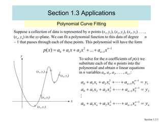
1. Section 1.3 Applications Polynomial Curve Fitting Section 1.3.1 Suppose a collection of data is represented by n points ( x 1 , y 1 ), ( x 2 , y 2 ), ( x 3 , y 3 ) . . . , ( x n , y n ) in the xy -plane. We can fit a polynomial function to this data of degree n – 1 that passes through each of these points. This polynomial will have the form y To solve for the n coefficients of p ( x ) we substitute each of the n points into the polynomial and obtain n linear equations in n variables a 0 , a 1 , a 2 , . . . , a n -1 : ( x 1 , y 1 ) ( x 2 , y 2 ) ( x 3 , y 3 ) ( x n , y n ) x
2. Section 1.3 Applications Polynomial Curve Fitting Section 1.3.2 Example 1 : The graph of a cubic polynomial has horizontal tangents at (1, – 2) and (– 1, 2). Find the equation for the cubic and sketch its graph. Solution : The general form for a cubic polynomial is The derivative of this function is We know the derivative is zero at the given points so we obtain the equations
3. Section 1.3 Applications Polynomial Curve Fitting Section 1.3.3 Example 1 : These substitutions lead to the following system of equations Which in turn leads to the augmented matrix We now solve this system:
4. Section 1.3 Applications Polynomial Curve Fitting Section 1.3.4 Example 1 : From this matrix we have a 2 = 0 and a 1 = – 3 a 3 . Now using the given points and the solutions from the above system we substitute into equation (1) to obtain: or This is a new system of equations with augmented matrix:
5. Section 1.3 Applications Polynomial Curve Fitting Section 1.3.5 Example 1 : We now solve this system: From the last matrix we see that a 0 = 0 and a 3 = 1, and consequently a 1 = – 3. The equation of the polynomial is p ( x ) = – 3 x + x 3 . We can now sketch the graph of the third degree polynomial that goes through these points and has horizontal tangents at these points.
6. Section 1.3 Applications Polynomial Curve Fitting Example 1 : We now graph the polynomial p ( x ) = – 3 x + x 3 : ( – 1, 2) ( 1, – 2) Section 1.3.6
7. Section 1.3 Applications Network Analysis Section 1.3.7 Networks composed of branches and junctions are used as models in fields as diverse as economics, traffic analysis, and electrical engineering. It is assumed in such models that the total flow into a junction is equal to the total flow out of the junction. For example, because the junction shown below has 30 units flowing into it, there must be 30 units flowing out of it. We show this diagrammatically as and can be represented by the linear system Since we can represent each junction in a network gives rise to a linear equation we can analyze the flow through a network composed of several junctions by solving a system of linear equations. 30 x 1 x 2
8.
9. Section 1.3 Applications Network Analysis Section 1.3.9 Example 2 : We label each junction appropriately as shown. We then establish the equations: Junction 1 Junction 2 Junction 3 Junction 4 These equations lead to the following system of linear equations: 200 100 100 200 x 1 x 3 x 2 x 4 1 2 3 4
10. Section 1.3 Applications Network Analysis Section 1.3.10 Example 2 : This system of linear equations leads to the following matrix representation: We now use the Gauss-Jordan elimination technique to solve this system.
11. Section 1.3 Applications Network Analysis Section 1.3.11 Example 2 : From the fourth row we see that x 4 can be any real number, so letting x 4 = t we have the following general solution: x 4 = t , x 3 = 200 + t , x 2 = t – 100 , x 1 = 100 + t where t is a real number. Thus this system has an infinite number of solutions. This is the solution to part (a) of the question.
12.
13.
14. Section 1.3 Applications Analysis of an Electrical Network Section 1.3.14 Example 3 : Determine the currents I 1 , I 2 , and I 3 or the electrical network shown below. 1 2 Path 1 Path 2 8 Volts 7 Volts R 3 = 4 R 2 = 2 R 1 = 3 I 1 I 2 I 3