NCompass Live - Aug. 22, 2018 http://nlc.nebraska.gov/ncompasslive/ Microsoft Excel has a variety of uses in the library world from keeping track of budgets or managing program registrations to viewing circulation or collection statistics. Learn some hints and tips for working with already existing spreadsheets as well as building your own. We’ll also take a look at Google Sheets and see how that compares with Excel. Presenter: Megan Boggs, Seward (NE) Memorial Library.

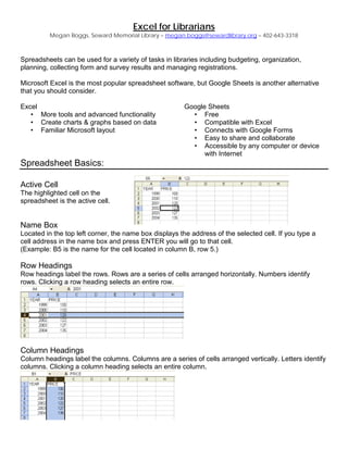
1. Excel for Librarians
Megan Boggs, Seward Memorial Library – megan.boggs@sewardlibrary.org – 402-643-3318
Spreadsheets can be used for a variety of tasks in libraries including budgeting, organization,
planning, collecting form and survey results and managing registrations.
Microsoft Excel is the most popular spreadsheet software, but Google Sheets is another alternative
that you should consider.
Excel
• More tools and advanced functionality
• Create charts & graphs based on data
• Familiar Microsoft layout
Google Sheets
• Free
• Compatible with Excel
• Connects with Google Forms
• Easy to share and collaborate
• Accessible by any computer or device
with Internet
Spreadsheet Basics:
Active Cell
The highlighted cell on the
spreadsheet is the active cell.
Name Box
Located in the top left corner, the name box displays the address of the selected cell. If you type a
cell address in the name box and press ENTER you will go to that cell.
(Example: B5 is the name for the cell located in column B, row 5.)
Row Headings
Row headings label the rows. Rows are a series of cells arranged horizontally. Numbers identify
rows. Clicking a row heading selects an entire row.
Column Headings
Column headings label the columns. Columns are a series of cells arranged vertically. Letters identify
columns. Clicking a column heading selects an entire column.

2. Formula Bar
Located on the top of the spreadsheet, below
the toolbars, the formula bar displays text
from the selected cell. If there is a formula in
the cell, the formula, not the answer to the
formula, is displayed in the formula bar.
Clicking on the symbol next to the formula
bar will assist you in entering formulas.
Formulas
A formula will instruct Excel to automatically do something (add, multiply, average, etc.) to a set of
cells. To begin writing a formula in the formula bar, you must first type an equal sign.
Example formula:
To put the total of cells A3, A4 and A5 into cell A7 you would click in cell A7 and type in the formula
bar =A3+A4+A5
Hint: When entering formulas, after you type an equal sign, instead of typing the cell names (A3, A4)
click the cell you want to sum. All formulas start with an = sign.
Functions:
These formulas are used for working with long lists of numbers. A typical function looks like this:
=SUM(A3:A30)
• SUM is a function, meaning that it sums (adds up) the list of numbers.
• The list of numbers is indicated in brackets.
• The address of the first cell in the list is A3.
• A colon : separates this cell address from the last cell in the list, which is A30.
More Spreadsheet Tips & Tricks:
Freezing Panes
Without the headings, it’s hard to keep track of which column or row of data you are looking at. To
avoid this problem use the freeze panes to "freeze" certain areas or panes of the spreadsheet so that
they remain visible at all times when scrolling to the right or down. Keeping headings on the screen
makes it easier to read your data throughout the entire spreadsheet. When you activate Freeze
Panes (found in the “View” tab of the ribbon) in Excel, all the rows above the active cell and all the
columns to the left of the active cell become frozen.
Sorting
Excel's sort feature (found in the “Data” tab of the ribbon) is a quick and easy way to sort data in a
spreadsheet. The options for sorting your data include:
• Sort in ascending order - A to Z alphabetically or smallest to largest for number data.
• Sort in descending order - Z to A alphabetically or largest to smallest for number data.

3. Customizing Worksheet Tabs
Right-clicking on any of the worksheet tabs at the bottom of your spreadsheet allows you to
customize them. Two of the most popular options are:
• Rename
• Tab Color
Referencing Another Worksheet
Click the cell in which you want to enter the formula. In the formula bar, type = (equal sign) and the
formula you want to use. Click the tab for the worksheet to be referenced. Select the cell or range of
cells to be referenced.
=SUM(Sheet1!A1:A5) Using this example formula, you could put the total sum of cells A1 through A5
from Sheet1 into a cell on Sheet2.
Fill Handle
When you want to save time filling in content on a spreadsheet try using the fill handle! Hover over
the small black square in the bottom right corner of the active cell until you see a black cross. Then
click and drag down or to the right to copy and fill. This can be used in many ways!
Add More Than One New Row or Column
Instead of inserting rows or columns one by one you can drag and select however many rows or
columns you want to add above or to the left. Right click the highlighted rows or columns and choose
Insert from the drop down menu. New rows will be inserted above the row or to the left of the column
you first selected.
Bottom Status Bar
After selecting a range of cells, look at the bottom right gray bar on the workbook to check things like
SUM, COUNT, and AVERAGE. Right click for more options.
Locking Reference Cells
It’s important to understand the difference between relative, absolute and mixed cell references.
Unlike relative references, absolute references do not change when copied or filled. You can
use an absolute reference to keep a row and/or column constant. When typing a formula or function
you can make a cell absolute by adding dollar signs before the row and column heading. Example:
A2 is relative, $A$2 is absolute, A$2 or $A2 is mixed.
Printing Options
When printing a spreadsheet you can choose to print just selected areas, a whole sheet or an entire
workbook. You can access additional printing options by clicking on Page Layout > Page Setup.
Additional options include:
• Page orientation
• Scaling
• Margins
• Header and footer
• Gridlines
• Row and column headings

4. Hyperlinks in Spreadsheets
When typing website or email addresses into a spreadsheet, they will automatically be converted into
hyperlinks. If you would like to turn this option off you can do so by finding the AutoCorrect Options in
the File Menu under Excel Options > Proofing. Click on the AutoFormat As You Type tab and then
uncheck the “Internet and network paths with hyperlinks” box.
Display Text in Multiple Lines
When entering text into the cell, press Alt-Enter to insert a line break.
To reformat existing cells so they have wrapped text, select the cells and then choose Format >
Format Cells. On the Alignment tab, select "wrap text," and click OK.
Adjust Text Orientation
Sometimes it’s helpful to rotate the direction of the text to be able to compress the
width of a column. You can do this by using the Orientation tool on the Home ribbon or
by choosing Format > Format Cells.
Transpose data from a row to a column
After working with the data for a while, you decide you'd rather have the current set of row labels
running across the columns. Don’t worry about re-keying the data, just copy the information and use
“transpose” under the Paste Special option.
COUNTIF Function
When compiling spreadsheet data, especially when looking at results of surveys, it’s great to be able
to use the COUNTIF Function to total up various responses. Find a blank area of the spreadsheet to
put your totals and then enter =COUNTIF(A2:A11,”always”) in the cell. The A2:A11 would be the
range of cells where you are getting your results from and the word or set of words in quotation marks
is what you will be totaling.