Oltre l'orizzonte cosmologico
•
0 likes•2,342 views

Seminario del Prof. Paolo de Bernardis 11 Marzo 2010 Aula A Dipartimento di Fisica ore 13.15

Recommended
More Related Content
What's hot
What's hot (19)
Viewers also liked
Viewers also liked (10)
Similar to Oltre l'orizzonte cosmologico
Similar to Oltre l'orizzonte cosmologico (20)
More from nipslab
More from nipslab (15)
Oltre l'orizzonte cosmologico
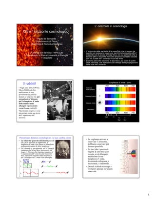
- 1. L’ orizzonte in cosmologia Oltre l’ orizzonte cosmologico Paolo de Bernardis Dipartimento di Fisica Università di Roma La Sapienza • L’ orizzonte delle particelle è la superficie che ci separa da A pranzo con la fisica - NIPS Lab quanto non possiamo osservare, perché la luce partita oltre l’ Dipartimento di Fisica Università di Perugia orizzonte non è ancora arrivata fino a noi. Le particelle che si trovano oltre l’ orizzonte non sono ancora in contatto causale 11/03/2010 con noi. Esiste se l’ universo ha un’età finita. • Esistono però altri orizzonti, di tipo fisico, più vicini di quello delle particelle, che dipendono dai dettagli della propagazione della luce nell’ universo. Lunghezza d’ onda λ (nm) Il redshift • Negli anni ’20 Carl Wirtz, Galassia Edwin Hubble ed altri, molto lontana analizzarono la luce proveniente da galassie distanti, e notarono che piu’ Galassia lontana una galassia e’ distante, piu’ le lunghezze d’ onda della sua luce sono Galassia vicina allungate (spostamento verso il rosso, redshift). laboratorio •Questo dato empirico viene interpretato come una prova dell’ espansione dell’ Ca II HI universo. Mg I Na I Percorrendo distanze cosmologiche, la luce cambia colore • Se vogliamo arrivare a • La relativita’ generale di Einstein prevede che, in un universo in espansione, le osservare l’ orizzonte, lunghezze d’onda λ dei fotoni si allunghino dobbiamo osservare più esattamente quanto le altre lunghezze. lontano possibile. • Piu’ distante e’ una galassia, piu’ e’ lungo il cammino che la luce deve percorrere, piu’ • La luce che è partita da lungo e’ il tempo che impiega, maggiore e’ regioni di universo così l’ espansione dell’ universo dal momento remote, avrà allungato dell’ emissione a quello dalla ricezione, e piu’ la lunghezza d’ onda viene allungata. moltissimo le sue lunghezze d’ onda, to diventando infrarossa, o microonde, o radioonde … t1 • Quindi richiede telescopi e rivelatori speciali per essere osservata. t2 1
- 2. • L’ orizzonte a cui si arriva, però, è di tipo fisico. Orizzonte fisico • Infatti l’ espansione dell’ universo comporta un suo • In un universo in espansione, dominato dalla raffreddamento. Osservando lontano riceveremo radiazione, si può calcolare accuratamente il luce che è stata emessa quando l’ universo era più tempo necessario per passare dal Big Bang caldo di oggi. (densità e temperatura infinite) fino alla • Se guardiamo abbastanza lontano, arriveremo ad temperatura in cui elettroni e protoni osservare epoche in cui l’ universo era caldo come possono combinarsi in atomi (ricombinazione dell’ idrogeno). o più della superficie del sole. • La temperatura a cui avviene la • E quindi era ionizzato. In quell’ epoca i fotoni non ricombinazione è circa 3000K, e il tempo potevano propagarsi su linee rette, ma su spezzate necessario per arrivarci è di 380000 anni. venendo continuamente diffusi dagli elettroni liberi • Quindi per i primi 380000 anni della sua del mezzo ionizzato. evoluzione l’ universo è ionizzato e opaco. • L’ universo primordiale è opaco, come opaco è l’ interno di una stella. Orizzonte fisico Composizione della luce che viene dal sole (spettro) Lunghezza d’ onda (micron) • Osservando sempre più lontano, potremo vedere solo finchè l’ universo è Intensità luminosa W/m2/sr/cm-1) Radiazione Termica, trasparente. Cioè fino all’ epoca della Spettro di Corpo Nero ricombinazione. • Possiamo quindi osservare entro un orizzonte che è una superficie sferica, centrata sulla nostra posizione, al di là della quale l’ universo è opaco a causa delle diffusioni (scattering) contro gli elettroni liberi subite dai fotoni. • Si chiama superficie di ultimo scattering ed è il nostro orizzonte fisico. Strong evidence for a hot early phase of the Universe Orizzonte fisico • Nel seguito: Thermal spectrum …. –L’ osservazione della superficie di … and accurate isotropy ultimo scattering. • Come si fa 0K 3K 5K • Quali sono i risultati • Orizzonti causali impressi nell’ orizzonte fisico • Conseguenze per la cosmologia e la Cosmic fisica fondamentale Microwave –Come andare oltre. Background 2
- 3. How to detect CMB photons How to detect CMB photons • E(γCMB) of the order of 1 meV • E(γCMB) of the order of 1 meV • Frequency: 15-600 GHz • Frequency: 15-600 GHz • Detection methods: • Detection methods: – Coherent (antenna + amplifier) – Coherent (antenna + amplifier) – Thermal (bolometers) – Thermal (bolometers) – Direct (Cooper pairs in KIDs) – Direct (Cooper pairs in KIDs) • Space (atmospheric opacity) • Space (atmospheric opacity) Cryogenic Bolometers Cryogenic Bolometers Again, need • The CMB spectrum is a continuum and bolometers are wide band • Johnson noise in the thermistor of low detectors. That’s why they are so sensitive. temperature d Δ V J2 and low Thermometer = 4 kTR (Ge thermistor (ΔR) df background Load resistor at low T) • Temperature noise d Δ W T2 4 kT 2 G eff = 2 df G eff + (2π fC ) 2 Incoming Q ΔV Photons (ΔB) • Photon noise d ΔWPh 4k 5TBG x4 (ex −1+ ε ) 2 5 Feed = 2 3 ∫ε dx Integrating Horn filter df ch (ex −1)2 Radiation cavity (angle selective) (frequency • Total NEP (fundamental): Absorber (ΔT) selective) 1 d ΔVJ d ΔWT d ΔWPh 2 2 2 • Fundamental noise sources are Johnson noise in the thermistor (<ΔV2> = 4kTRΔf), temperature fluctuations in the thermistor NEP2 = + + ((<ΔW2> = 4kGT2Δf), background radiation noise (Tbkg5) need ℜ2 df df df to reduce the temperature of the detector and the radiative background. •The absorber is micro machined as a web of Spider-Web Bolometers metallized Si3N4 wires, 2 μm thick, with 0.1 mm Built by JPL Signal wire pitch. Absorber •This is a good absorber for mm-wave photons and features a very low cross section for cosmic rays. Circa 1970 Also, the heat capacity is reduced by a large factor with respect to the solid absorber. Circa 1980 •NEP ~ 2 10-17 W/Hz0.5 is achieved @0.3K •150μKCMB in 1 s •Mauskopf et al. Appl.Opt. Thermistor 36, 765-771, (1997) 2 mm 3
- 4. Development of thermal detectors for far IR and mm-waves 17 10 How to detect CMB photons Langley's bolometer Golay Cell a measurement (seconds) 12 • E(γCMB) of the order of 1 meV 10 Golay Cell time required to make Boyle and Rodgers bolometer • Frequency: 15-600 GHz 1year F.J.Low's cryogenic bolometer • Detection methods: 7 10 Composite bolometer 1day – Coherent (antenna + amplifier) 1 hour Composite bolometer at 0.3K – Thermal (bolometers) 2 10 – Direct (Cooper pairs in KIDs) 1 second Spider web bolometer at 0.3K Spider web bolometer at 0.1K Photon noise limit for the CMB • Space (atmospheric opacity) 1900 1920 1940 1960 1980 2000 2020 2040 2060 year COBE-FIRAS MPI • COBE-FIRAS was a (Martin Puplett cryogenic Martin- Interferometer) Puplett Fourier- Beamsplitter = Transform wire grid polarizer Spectrometer with composite Differential bolometers. It was instrument placed in a 400 km orbit. • A zero instrument ∞ I SKY ( x) = C ∫ [SSKY (σ ) − SREF (σ )]rt(σ ){ + cos[4πσx]}dσ 1 comparing the specific sky brightness to the 0 ∞ brightness of a ICAL( x) = C∫ [SCAL(σ ) − SREF (σ )]rt(σ ){ + cos[4πσx]}dσ 1 cryogenic Blackbody 0 FIRAS • The FIRAS guys were able to change the temperature of the internal blackbody until the interferograms were null. • This is a null measurement, which is much more sensitive than an absolute one: (one can boost the gain of the instrument without saturating it !). • This means that the difference between the spectrum of the sky and the spectrum of a blackbody is zero, i.e. the spectrum of the sky is a blackbody with that temperature. • This also means that the internal blackbody is a real blackbody: it is unlikely that the sky can have the same deviation from the Planck law characteristic of the source built in the lab. σ (cm-1) wavenumber 4
- 5. • The spectrum • Techniques ? 2h ν 3 B(ν , T ) = c2 ex −1 TCMB = 2.725K RJ Wien RJ Wien hν ν xCMB = ≅ kTCMB 56 GHz xmax 1 − e − xmax = ⇒ xmax = 2.82 ⇒ 3 ν << ν max = 160 GHz ⇒ coherent detectors ν max = 159 GHz (σ max = 5.31 cm −1 ) ν >> ν max = 160 GHz ⇒ bolometers λ B(ν , T ) = B(λ , T ) ⇒ λmax = 1.06 mm ν ≈ ν max = 160 GHz ⇒ ? ?? ν • The DMR instrument aboard of the COBE satellite COBE-DMR CMB anisotropy Cosmic Horizons measured the first map of • The very good isotropy of the CMB sky is to CMB anisotropy (1992) some extent surprising. Galactic Plane • The contrast of the image is very low, but there are • The CMB comes from an epoch of 380000 years structures, at a level of after the Big Bang. 10ppm. • So it depicts a region of the universe as it was • Instrumental noise is 380000 years after the Big Bang. significant in the maps (compare the three different • The region we can map, however, is much wider wavelengths) than 380000 light years. • DMR did not have a real • So it contains subregions which are separated telescope, so the angular more than the length light has travelled since the resolution was quite coarse Big Bang. These regions would not be in causal (10 o !!) contact in a static universe. R= distance from R= distance from us = 14 Glyrs a l Gly us = 14 Glyrs s ev er y 4 Gl But also distance in But also distance in R=1 R time: 14 Gyrs ago R= time: 14 Gyrs ago & 14 t Gl y here, now here, now K K 000 000 T=3 T=3 Transparent Transparent universe universe Opaque Opaque universe universe 5
- 6. Cosmic Horizons r=3 R= distance from 80 k l y ly us = 14 Glyrs er al G ly s ev 0k • We measure the same brightness y 38 4 Gl But also distance in r= (temperature) in all these regions, and this R=1 R= time: 14 Gyrs ago 14 Gl is surprising, because to attain thermal y equilibrium, contact is required ! (through forces, thermal, radiative …). here, now • We live in an expanding universe. Regions K separated by more than 380000 light 000 T=3 years might have been in causal contact Transparent Opaque universe (and thus homogeneized) earlier. universe Expansion vs Horizon Expansion vs Horizon In a Universe made of on In a Universe made of on r iz r iz matter and radiation, the e ho matter and radiation, the e ho expansion rate decreases f th expansion rate decreases f th with time. eo with time. eo s iz s iz size of size of ed region ed region the consider the consider So a region as large as the horizon when the CMB is released …. 380000 y time time Expansion vs Horizon Expansion vs Horizon In a Universe made of on In a Universe made of on r iz r iz matter and radiation, the e ho matter and radiation, the e ho expansion rate decreases f th expansion rate decreases f th with time. eo with time. eo s iz s iz size of size of ed region ed region the consider the consider … has never been … nor has been causally connected causally connected to before surrounding regions 380000 y 380000 y time time 6
- 7. Cosmic Horizons Granulazione solare • Hence the “Paradox of Horizons” : Gas incandescente sulla superficie del • We see approximately the same temperature Sole (5500 K) everywhere in the map of the CMB, but we 8 minuti luce Qui, ora do not understand how this has been obtained in the first 380000 years of the evolution of the universe. • Was this temperature regulated everywhere ab-initio ? • Are our assumptions about the composition of the universe wrong, and the universe does not decelerate in the first 380000 years ? Granulazione solare Flatness Paradox Gas incandescente • The expansion of the Universe is regulated by the sulla superficie del Friedmann equation, directly deriving from Sole (5500 K) Einstein’s equations for a homogeneous and Qui, ora 8 minuti luce isotropic fluid. • If the Universe contains only matter and radiation, it either collapses or dilutes, with a rate depending on Gas incandescente the mass-energy density. nell’ universo primordiale (l’ • To get an evolution with a mass-energy density of universo diventa the order of the observed one today, billions of trasparente a 3000 K) years after the Big Bang, you need to tune it at the Qui, ora 14 miliardi di anni luce beginning very accurately, precisely equal to a critical value. Mappa di BOOMERanG dell’ Universo Primordiale • How was this fine-tuning achieved ? Inflation might be the solution a(t) C I n os m fla ic tio n Sub-atomic scales ang ig B th eB ter t=10-36s s af Cosmic distances 1n ity, Quantum fluctuations of ens ic al d the field dominating the Crit energy of the universe Energy scale: 1016 GeV Cosmic Inflation: A very fast expansion Cosmological scales of the universe, driven by a phase transition in t=380000 y Billion years t the first split-second density fluctuations 7
- 8. ma l size of d region Expansion vs Horizon nor lution the considere e vo According to the inflation on on r iz r iz theory …. e ho e ho f th f th eo eo s iz s iz exponential size of expansion ed region the consider Inflation: A region as large as the horizon when the CMB is released …. …had been causally connected to the surrounding regions before inflation 380000 y 10-36 s time time ma l size of d region • Inflation nor lution the considere – Provides a physical process to origin density fluctuations e vo – Explains the flatness paradox – Explains the horizons paradox on r iz • Is a predictive theory (a list of > models has been compiled..) e ho f th – Predicts gaussian density fluctuations eo – Predicts scale invariant density fluctuations s iz – Predicts Ω=1 exponential • How can we test it ? expansion Inflation: • We still expect a difference between the physical processes happening inside the horizon and those relevant outside the horizon. • So we expect anyway that the scale of the causal horizon is Here the horizon imprinted in the image of the CMB. contains all of the • The angular size subtended by the horizons when the CMB is universe observable released is around 1 degree, if the geometry of space is today Euclidean. • We need sharp images of the CMB, so that we can resolve 10-36 s time the density fuctuations predicted by inflation. 380000 lyrs R θ d 1o R COBE resolution Here, now K 10o 000 (T= ng ∞) a BigB T=3 d ao 380000 ly θ≈ × ≈ ×1100 ≈1o R a 14000000000 ly R= distance from us = 14 Glyrs 8
- 9. LSS high resolution 14 Gly horizon • The images from COBE-DMR were not sharp Critical density Universe Ω=1 enough to resolve cosmic horizons (the angular 1o resolution was 7°). • After COBE, experimentalists worked hard to develop higher resolution experiments. • In addition to testing inflation, we expected high horizon resolution observations to give informations Ω>1 about 2o High density Universe a) The geometry of space b) The physics of the primeval fireball. horizon a) The angle subteneded by the horizon can be 0.5o more or less than 1° if space is curved. Low density Universe Ω<1 PS PS PS The quest for high resolution 0 200 High density Universe l 0 200 Critical density Universe l 0 200 Low density Universe l b) Within a causally connected region, the Ω>1 Ω=1 Ω<1 hot, ionized gas of the primeval fireball is subject to opposite forces: gravity and photon pressure. 2o 1o • If a density fluctuation is present, 0.5o “acoustic oscillations” start, depending on the composition of the universe (density of baryons) and on the spectrum of initial density fluctuations. Density perturbations (Δρ/ρ) were oscillating in the primeval plasma (as a result of the opposite effects of gravity and photon pressure). Due to gravity, T is reduced enough Δρ/ρ increases, that gravity wins again • The study of solar oscillations and so does T allows us to study the interior structure of the sun, well below the photosphere, because these waves depend on the internal Pressure of photons structure of the sun. overdensity increases, resisting to the compression, and the t perturbation bounces back • The study of CMB anisotropy Before recombination T > 3000 K allows us to study the universe t After recombination T < 3000 K well behind (well before) the cosmic photosphere (the Here photons are not tightly recombination epoch), because coupled to matter, and their the oscillations depend on the pressure is not effective. composition of the universe Perturbations can grow and form Galaxies. and on the initial perturbations. After recombination, density perturbation can grow and create the hierarchy of structures we see in the nearby Universe. 9
- 10. How to obtain wide, high angular How to obtain wide, high angular resolution maps of the CMB resolution maps of the CMB • Angular Resolution: Microwave telescope, at • Angular Resolution: Microwave telescope, at relatively high frequencies (θ=λ/D) relatively high frequencies (θ=λ/D) • 150GHz: peak of CMB brightness • 150GHz: peak of CMB brightness • Low sky noise and high transparency at 150 GHz: • Low sky noise and high transparency at 150 GHz: Balloon or Satellite Balloon or Satellite • High sensitivity at 150 GHz: cryogenic bolometers • High sensitivity at 150 GHz: cryogenic bolometers • Multiband for controlling foreground emission • Multiband for controlling foreground emission • Sensitivity and sky coverage (size of explored Statistical samples of the CMB sky (about one hundred directions) in the 90s region): either – Extremely high sensitivity (0.1K) and regular flight In Italy: ARGO In the USA: MAX, MSAM, … or – High sensitivity (0.3K) and long duration flight How to obtain wide, high angular Universita’ di Roma, La Sapienza: Cardiff University: P. Ade, P. Mauskopf P. de Bernardis, G. De Troia, A. Iacoangeli, IFAC-CNR: A. Boscaleri S. Masi, A. Melchiorri, L. Nati, F. Nati, F. INGV: G. Romeo, G. di Stefano resolution maps of the CMB Piacentini, G. Polenta, S. Ricciardi, P. Santini, M. Veneziani IPAC: B. Crill, E. Hivon CITA: D. Bond, S. Prunet, D. Pogosyan Case Western Reserve University: • Angular Resolution: Microwave telescope, at J. Ruhl, T. Kisner, E. Torbet, T. Montroy LBNL, UC Berkeley: J. Borrill Imperial College: A. Jaffe, C. Contaldi relatively high frequencies (θ=λ/D) Caltech/JPL: A. Lange, J. Bock, W. Jones, V. Hristov U. Penn.: M. Tegmark, A. de Oliveira-Costa Universita’ di Roma, Tor Vergata: N. Vittorio, • 150GHz: peak of CMB brightness University of Toronto: B. Netterfield, C. MacTavish, E. Pascale G. de Gasperis, P. Natoli, P. Cabella • Low sky noise and high transparency at 150 GHz: Balloon or Satellite • High sensitivity at 150 GHz: cryogenic bolometers • Multiband for controlling foreground emission • Sensitivity and sky coverage (size of explored region): either – Extremely high sensitivity (0.1K) and regular flight MAXIMA or – High sensitivity (0.3K) and long duration flight BOOMERanG BOOMERanG the BOOMERanG ballon-borne telescope 120 mm 3He Sun Shield fridge Solar Array Differential GPS Array D D Star Camera Cryostat and 0.3K detectors D D D D D Focal plane assembly Ground BOOMERanG-LDB Appl.Opt Shield Primary 1.6K MultiBand Mirror 150 D = location of detectors Photometers 150 (150,240,410) (1.3m) preamps 90 90 4o on the sky Sensitive at 90, 150, 240, 410 GHz 10
- 11. • The instrument is flown 9/Jan/1999 above the Earth atmosphere, at an altitude of 37 km, by means of a stratospheric balloon. • Long duration flights (LDB, 1-3 weeks) are performad by NASA-NSBF over Antarctica • BOOMERanG has been flown LDB two times: • From Dec.28, 1998 to Jan.8, 1999, for CMB anisotropy measurements • In 2003, from Jan.6 to Jan.20, for CMB polarization measurements (B2K). BOOMERanG • 1998: • 1998: BOOMERanG BOOMERanG mapped the mapped the temperature temperature fluctuations of fluctuations of the CMB at the CMB at sub-horizon sub-horizon scales (<1O). scales (<1O). • The signal • The rms was well signal has the above the CMB noise: spectrum and does not fit 2 indep. det. at 150 GHz any spectrum of foreground emission. PS PS PS 0 200 l 0 200 l 0 200 l High density Universe Critical density Universe Low density Universe Ω>1 Ω=1 Ω<1 2o 1o 0.5o 11
- 12. In the primeval plasma, photons/baryons density perturbations start to oscillate only when the sound horizon becomes larger than their linear size . Small wavelength perturbations oscillate faster than large ones. Full power multipole The angle subtended depends on the geometry of space spectrum Size of sound horizon v v v LSS measurement 2nd dip from C R BOOMERanG size of perturbation (2002) (wavelength/2) v v 450 -Geometry of C R 2nd peak the universe from location of v v first peak C 1st dip -Signature of v 380000 ly inflation from amplitudes of 3 220 C 1st peak peaks and general slope 0y time 300000 y Big-bang recombination Power Spectrum We can measure cosmological parameters with CMB ! Temperature Angular spectrum varies with Ωtot , Ωb , Ωc, Λ, τ, h, ns, … “The perfect universe” • Data consistent with flat Universe Radiation Normal Matter • Baryon fraction agrees with BBN < 0.3% 4% • With supernovae or LSS => Λ term Dark Matter 22% Dark Energy 74% 12
- 13. Did Inflation really happen ? CMB polarization • We do not know. Inflation has not been • CMB radiation is Thomson scattered at recombination. proven yet. It is, however, a mechanism able • If the local distribution of incoming radiation in the to produce primordial fluctuations with the right rest frame of the electron has a quadrupole moment, characteristics. the scattered radiation acquires some degree of linear polarization. • Four of the basic predictions of inflation have been proven: Last scatte ri ng surface – existence of super-horizon fluctuations – gaussianity of the fluctuations – flatness of the universe – scale invariance of the density perturbations • One more remains to be proved: the stochastic background of gravitational waves produced during the inflation phase. • CMB can help in this – see below. y y - -10ppm +10ppm + If inflation really happened… x x + - + - - - • It stretched geometry of OK space to nearly Euclidean y - + • It produced a nearly scale invariant spectrum of density OK fluctuations x - • It produced a stochastic background of gravitational waves. ? = e- at last scattering Quadrupole from P.G.W. B-modes from P.G.W. • If inflation really happened: • The amplitude of this effect is very small, but It stretched geometry of space to depends on the Energy scale of inflation. In fact the nearly Euclidean amplitude of tensor modes normalized to the scalar It produced a nearly scale invariant ones is: 1/ 4 spectrum of gaussian density 1/ 4 ⎛ C2 ⎞ GW Inflation potential ⎛T ⎞ V 1/ 4 fluctuations ⎜ ⎟ ≡ ⎜ Scalar ⎟ ⎜C ⎟ ≅ It produced a stochastic background of ⎝S⎠ ⎝ 2 ⎠ 3.7 × 10¹⁶ GeV gravitational waves: Primordial G.W. • and l(l + 1) B ⎡ V 1/ 4 ⎤ The background is so faint that even E-modes cl max ≅ 0.1μK ⎢ ⎥ LISA will not be able to measure it. 2π ⎢ ⎣ 2 ×10¹⁶ GeV ⎥ ⎦ • Tensor perturbations also produce • There are theoretical arguments to expect that the quadrupole anisotropy. They generate energy scale of inflation is close to the scale of GUT irrotational (E-modes) and rotational (B-modes) components in the CMB i.e. around 1016 GeV. polarization field. • The current upper limit on anisotropy at large scales • Since B-modes are not produced by scalar gives T/S<0.5 (at 2σ) fluctuations, they represent a signature of • A competing effect is lensing of E-modes, which is inflation. B-modes important at large multipoles. 13
- 14. PSB devices & feed optics (Caltech + JPL) PSB Pair 06/01/2003 145 GHz B03 TT Power Spectrum T map • Detection of anisotropy signals all the way up to l=1500 (Masi et al., • Time and detector jacknife tests OK 2005) • Systematic effects negligible wrt noise & cosmic variance the deepest CMB map ever [Masi et al. 2005] Jones et al. 2005 19/20 TE Power Spectrum • Smaller signal, but detection evident (3.5σ) • NA and IT results consistent • Error bars dominated by cosmic variance • Time and detectors Piacentini et al. 2005 jacknife OK, i.e. systematics negligible • Data consistent with TT best fit model La mappa dell’ universo primordiale con sovrapposta la polarizzazione Realizzata dal gruppo di Cosmologia di Tor Vergata (Genn. 2005) 14
- 15. EE Power Spectrum WMAP (2002) • Signal extremely small, but detection evident for EE Wilkinson Microwave Anisotropy Probe (non zero at 4.8σ). • No detection for BB nor for EB • Time and detectors jacknife OK, i.e. systematics negligible • Data consistent with TT best Montroy et al. 2005 fit model • Error bars dominated by detector noise. Montroy et al. 2005 WMAP in L2 : sun, earth, moon are all WMAP Hinshaw et al. 2006 well behind the solar shield. astro-ph/0603451 Detailed Views of the 1o Recombination Epoch (z=1088, 13.7 Gyrs ago) BOOMERanG Masi et al. 2005 astro-ph/0507509 Paradigm of CMB anisotropies Power spectrum k l Processed by smaller than Power of CMB causal effects like spectrum of temperature horizon Acoustic oscillations Scales perturbations Radiation pressure fluctuations Gaussian, from photons resists gravitational INFLATION adiabatic Quantum (density) compression fluctuations horizon horizon horizon in the early Universe (ΔT/T) = (Δρ/ρ) /3 + (Δφ/c2)/3 P(k)=Akn l( l+1) cl – (v/c)•n larger than horizon Scales Unperturbed plasma neutral 2006 Hinshaw et al. 2006 0 Big-Bang 10-36s Inflation 3 min Nucleosynthesis 300000 yrs Recombination t 15
- 16. Cosmological Parameters Assume an adiabatic inflationary model, and compare with same weak prior on 0.5<h<0.9 WMAP BOOMERanG (100% of the sky, <1% gain (4% of the sky, 10% gain Need for high calibration, <1% beam, calibration, 10% beam, angular multipole coverage 2-700) multipole coverage 50- resolution 1000) Bennett et al. 2003 < 10’ Ruhl et al. astro-ph/0212229 • Ωο =1.02+0.02 • Ωο = 1.03+0.05 • ns = 0.99+0.04 * • ns = 1.02+0.07 • Ωbh2 =0.022+0.001 • Ωbh2 =0.023+0.003 • Ωmh2 =0.14+0.02 • Ωmh2 =0.14+0.04 • T = 13.7+0.2 Gyr • T=14.5+1.5 Gyr τrec= ? 2006 • • τrec= 0.166+0.076 Hinshaw et al. 2006 PLANCK 2009 Planck is a very ambitious experiment. ESA’s mission to map the Cosmic Microwave Background Image of the whole sky at wavelengths near the intensity It carries a peak of the CMB radiation, with complex CMB experiment (the state of the art, a • high instrument sensitivity (ΔT/T∼10-6) few years ago) all the way to L2, • high resolution (≈5 arcmin) • wide frequency coverage (25 GHz-950 GHz) improving the sensitivity wrt • high control of systematics WMAP by at least a factor 10, •Sensitivity to polarization extending the frequency Launch: 2009; payload module: 2 instruments + telescope coverage towards high • Low Frequency Instrument (LFI, uses HEMTs) frequencies by a factor about 10 • High Frequency Instrument (HFI, uses bolometers) • Telescope: primary (1.50x1.89 m ellipsoid) Galaxy CMB 16
- 17. Galaxy Galaxy CMB CMB Two Instruments: Low Frequency (LFI) and High Frequency (HFI) Spider Web and PSB Bolometers • Ultra-sensitive Technology • Tested on BOOMERanG (Piacentini et al. 2002, Crill et al. 2004, Masi et al. 2006) for bolometers, filters, horns, scan at 0.3K and on Archeops at 0.1K (Benoit et al. 2004). • Crucial role of balloon missions to get important science results, but also to validate satellite technology. 17
- 18. Measured performance of Planck HFI bolometers (0.1K) (Holmes et al., Appl. Optics, 47, 5997, 2008) Multi-moded = Photon noise limit Planck-Herschel Launch May 14, 2009 15:12 CEST Telescopio fuori asse, diametro specchio principale 1.8 m 18
- 19. Observing strategy The payload will work from L2, to Launch May 14th, 2009 avoid the emission of the Earth, of the Moon, of the Sun Boresight (85o from spin axis) Cruise May-June 2009 Field of view rotates at 1 rpm Calibrations, M Scan Ecliptic plane start July 2009 1 o/day E L2 HFI Verification / Calibration Plan e an m al pl ste c ht -sy FI fo SL) -flig b H su , C in (I AS LIGH, BEAM Main beam Far side lobes LIGH, BEAM Spectral response Time response LFER, SPIN Optical polarisation LIGH, POLC Thermo-optical coupling, bckgnd 01TO, 16TO, 4KTO Linearity 4KTO Absolute response LIGH Detection noise RW72, SPIN, NOIS Crosstalk XTLK Detection chain caract QECn, IVCF, IBTU, PHTU Numerical compression CPSE, CPVA Cryo chain setup 4KTU,16TU, 01TU Compatibility XTRA, NOIS Scanning ACMS [1.7arcmin] Solar AA SUNI [50%] 3 months after launch The sky explored by Planck so far (First Light Survey, 2 weeks) ● The launch was flawless and the transfer to final orbit was completed on 1 July ● All parts of the satellite survived launch and it is fully functional ● Coldest temperature (0.1 K) was reached on 3 July. The thermal behavior (static and dynamic) is as predicted from the ground. ● The instruments have been fully tuned and are in stable operations since 30 July ● All planned initial tests and measurements have been completed on 13 August ● Planck is now transitioning into routine operational mode Preview of data from the first-light survey (2 weeks of stable operation) 19
- 20. The sky explored by Planck so far (First Light Survey, 2 weeks) Galactic Plane 20
- 21. The sky explored by Planck in the First Light Survey, first 2 weeks High Galactic Latitude (CMB) 21