SlideShare a Scribd company logo
1 of 53
Download to read offline
Chord of Contact         y
                                 b
                                              T  x0 , y0 
                      -a                    a x

                                -b

From an external point T, two tangents may be drawn.
Chord of Contact
                                y
                                 b
                                         P x1 , y1 
                                                   T  x0 , y0 
                      -a                     a x

                                -b

From an external point T, two tangents may be drawn.
                             xx yy
   tangent at P has equation 12  12  1
                             a    b
Chord of Contact
                                y
                                 b
                                         P x1 , y1 
                                                   T  x0 , y0 
                      -a                     a x
                                          Q  x2 , y 2 
                                -b

From an external point T, two tangents may be drawn.
                             xx yy
   tangent at P has equation 12  12  1
                             a    b
                             xx y y
   tangent at Q has equation 22  22  1
                             a     b
Chord of Contact
                                y
                                 b
                                         P x1 , y1 
                                                   T  x0 , y0 
                      -a                     a x
                                          Q  x2 , y 2 
                                -b

From an external point T, two tangents may be drawn.
                             xx yy
   tangent at P has equation 12  12  1
                             a    b
                             xx y y
   tangent at Q has equation 22  22  1
Now T lies on both lines,    a     b
Chord of Contact
                              y
                               b
                                       P x1 , y1 
                                                 T  x0 , y0 
                     -a                    a x
                                        Q  x2 , y 2 
                              -b

From an external point T, two tangents may be drawn.
                              xx yy
   tangent at P has equation 12  12  1
                              a     b
                              xx y y
   tangent at Q has equation 22  22  1
Now T lies on both lines,     a      b
                          xx yy                x2 x0 y2 y0
                        1 2 0  1 2 0  1 and    2
                                                     2 1
                           a     b              a     b
y
                                                 x2 x0 y2 y0
                          b                              2 1
                                   P x1 , y1  a
                                                     2
                                                           b
                                             T  x0 , y0 
                -a                     a x
                                    Q  x2 , y 2          x1 x0 y1 y0
                                                                 2 1
                                                              2
                         -b                                 a     b


Thus P and Q both must lie on a line with equation;
                        x0 x y0 y
                          2
                             2 1
                        a    b
which must be the line PQ i.e. chord of contact

Similarly the chord of contact of the hyperbola has the equation;
                        x0 x y0 y
                          2
                             2 1
                        a    b
Rectangular Hyperbola             y
                                 c
                            P cp, 
                                 p     c
                                       Q cq, 
                                         q
                                             x
                 xy  c 2


 1) Show that equation PQ is x  pqy  c p  q  (1)
Rectangular Hyperbola                y
                                    c
                            P cp, 
                                    p        c
                                             Q cq, 
                             T  x0 , y0      q
                                                   x
                 xy  c 2


 1) Show that equation PQ is x  pqy  c p  q  (1)
                                 2cpq 2c 
 2) Show that T has coordinates       ,     
                                 p  q p  q
         2cpq                  2c
   x0                  y0 
         pq                  pq
Rectangular Hyperbola                  y
                                      c
                              P cp, 
                                      p        c
                                               Q cq, 
                               T  x0 , y0      q
                                                     x
                   xy  c 2


 1) Show that equation PQ is x  pqy  c p  q  (1)
                                    2cpq 2c 
 2) Show that T has coordinates           ,       
                                    p  q p  q
         2cpq                     2c
   x0                    y0 
         pq                     pq
   Substituting into (1); x   p  q x0 y  c p  q 
                                  2c
Rectangular Hyperbola                  y
                                      c
                              P cp, 
                                      p        c
                                               Q cq, 
                               T  x0 , y0      q
                                                     x
                   xy  c 2


 1) Show that equation PQ is x  pqy  c p  q  (1)
                                    2cpq 2c 
 2) Show that T has coordinates           ,        
                                    p  q p  q
         2cpq                     2c
   x0                    y0 
         pq                     pq
   Substituting into (1); x   p  q x0 y  c p  q 
                                  2c
                                    2cx0       2c 2
                                x        y
                                    2cy0        y0
Rectangular Hyperbola                  y
                                      c
                              P cp, 
                                      p        c
                                               Q cq, 
                               T  x0 , y0      q
                                                     x
                   xy  c 2


 1) Show that equation PQ is x  pqy  c p  q  (1)
                                    2cpq 2c 
 2) Show that T has coordinates           ,        
                                    p  q p  q
         2cpq                     2c
   x0                    y0 
         pq                     pq
   Substituting into (1); x   p  q x0 y  c p  q 
                                  2c
                                    2cx0       2c 2
                                x        y             xy0  x0 y  2c 2
                                    2cy0        y0
Geometric Properties
(1) The chord of contact from a point on the directrix is a focal
    chord.
Geometric Properties
(1) The chord of contact from a point on the directrix is a focal
    chord.
ellipse
                                             a , y  i.e. x  a
As T is on the directrix it has coordinates       0       0
                                             e               e
Geometric Properties
(1) The chord of contact from a point on the directrix is a focal
    chord.
ellipse
                                             a , y  i.e. x  a
As T is on the directrix it has coordinates       0        0
                                             e                  e
 chord of contact will have the equation;            a
                                                    x 
                                                       e   yy0  1
                                                      a2       b2
                                                         x yy0
                                                             2 1
                                                        ae b
Geometric Properties
(1) The chord of contact from a point on the directrix is a focal
    chord.
ellipse
                                             a , y  i.e. x  a
As T is on the directrix it has coordinates       0        0
                                             e                  e
 chord of contact will have the equation;            a
                                                    x 
                                                       e   yy0  1
                                                      a2       b2
                                                         x yy0
                                                             2 1
Substitute in focus (ae,0)                              ae b
     ae
          0  1 0
     ae
             1
Geometric Properties
(1) The chord of contact from a point on the directrix is a focal
    chord.
ellipse
As T is on the directrix it has coordinates    a , y  i.e. x  a
                                                      0        0
                                                e                  e
 chord of contact will have the equation;               a
                                                       x 
                                                          e   yy0  1
                                                         a2       b2
                                                            x yy0
                                                                2 1
Substitute in focus (ae,0)                                 ae b
     ae
          0  1 0           focus lies on chord of contact
     ae
                                 i.e. it is a focal chord
             1
(2) That part of the tangent between the point of contact and the
    directrix subtends a right angle at the corresponding focus.
                                       y
                                           Pa cos , b sin  
                                                                  T
                                             S                        x

                                                                     a
                                                                  x
                                                                     e
(2) That part of the tangent between the point of contact and the
    directrix subtends a right angle at the corresponding focus.
                                       y
                                           Pa cos , b sin  
                                                                  T

Prove: PST  90                            S                        x

                                                                     a
                                                                  x
                                                                     e
(2) That part of the tangent between the point of contact and the
     directrix subtends a right angle at the corresponding focus.
                                        y
                                            Pa cos , b sin  
                                                                   T

Prove: PST  90                             S                        x
                       x cos y sin 
equation of tangent is               1                              a
             a            a       b                                x
               cos                                                   e
          a            y sin 
when x  , e                  1
          e     a         b
(2) That part of the tangent between the point of contact and the
     directrix subtends a right angle at the corresponding focus.
                                          y
                                                Pa cos , b sin  
                                                                       T

Prove: PST  90                                 S                        x
                       x cos y sin 
equation of tangent is                  1                               a
             a            a         b                                  x
               cos                                                       e
          a            y sin 
when x  , e                  1
          e     a         b
               cos y sin 
                              1
                 e        b
                       y sin  e  cos
                               
                          b          e
                                 be  cos 
                             y
                                   e sin 
(2) That part of the tangent between the point of contact and the
     directrix subtends a right angle at the corresponding focus.
                                          y
                                                Pa cos , b sin  
                                                                       T

Prove: PST  90                                 S                        x
                       x cos y sin 
equation of tangent is                  1                               a
             a            a         b                                  x
               cos                                                       e
          a            y sin 
when x  , e                  1
          e     a         b
               cos y sin 
                              1
                 e        b
                       y sin  e  cos                    a be  cos  
                                                     T  ,
                                                                         
                          b          e                   e    e sin  
                                 be  cos 
                             y
                                   e sin 
b sin   0
mPS 
     a cos  ae
        b sin 
   
     acos  e 
b sin   0         be  cos 
mPS                                   0
     a cos  ae    mTS  e sin 
        b sin                 a
                                  ae
   
     acos  e               e
                          be  cos       e
                                      
                            e sin       a  ae 2
b sin   0         be  cos 
mPS                                      0
     a cos  ae    mTS  e sin 
        b sin                  a
                                    ae
   
     acos  e                 e
                          be  cos          e
                                         
                              e sin        a  ae 2
                           be  cos 
                        
                          a 1  e 2 sin 
                           be  cos 
                          2
                          a 1  e 2 
                                       sin 
                              a
b sin   0         be  cos 
mPS                                      0
     a cos  ae    mTS  e sin 
        b sin                  a
                                    ae
   
     acos  e                 e
                          be  cos          e
                                         
                              e sin        a  ae 2
                           be  cos 
                        
                          a 1  e 2 sin 
                            be  cos 
                          2
                           a 1  e 2 
                                        sin 
                               a
                           ae  cos 
                         
                             b sin 
b sin   0                    be  cos 
mPS                                                   0
       a cos  ae               mTS  e sin 
          b sin                             a
                                                 ae
     
       acos  e                            e
                                       be  cos          e
                                                      
                                           e sin        a  ae 2
                                        be  cos 
                                     
                                       a 1  e 2 sin 
                                        be  cos 
                                     2
                                      a 1  e 2 
                                                   sin 
                                           a
                                      ae  cos 
                                    
                                         b sin 
              b sin       ae  cos 
mPS  mTS               
            acos  e      b sin 
           1
b sin   0                  be  cos 
mPS                                                 0
       a cos  ae             mTS  e sin 
          b sin                           a
                                               ae
     
       acos  e                          e
                                     be  cos          e
                                                    
                                         e sin        a  ae 2
                                      be  cos 
                                   
                                     a 1  e 2 sin 
                                        be  cos 
                                     2
                                      a 1  e 2 
                                                   sin 
                                           a
                                      ae  cos 
                                    
                                         b sin 
              b sin       ae  cos 
mPS  mTS               
            acos  e      b sin                   PST  90
           1
(3) Reflection Property
    Tangent to an ellipse at a point P on it is equally inclined to
    the focal chords through P.
                       T                  y
                                               P
                                                                  T
                                      S        S                     x
(3) Reflection Property
      Tangent to an ellipse at a point P on it is equally inclined to
      the focal chords through P.
                         T                  y
                                                 P
                                                                    T
                                        S        S                     x


Prove: SPT  S PT 
(3) Reflection Property
       Tangent to an ellipse at a point P on it is equally inclined to
       the focal chords through P.
                          T                  y
                                                  P
                                                                     T
                                         S        S                     x


Prove: SPT  S PT 
  Construct a line || y axis passing through P
(3) Reflection Property
       Tangent to an ellipse at a point P on it is equally inclined to
       the focal chords through P.
                           T                  y
                                                      P
                      N                                             N
                                                                     T
                                          S          S                  x


Prove: SPT  S PT 
  Construct a line || y axis passing through P
   PT PN
                 (ratio of intercepts of || lines)
   PT  PN 
(3) Reflection Property
       Tangent to an ellipse at a point P on it is equally inclined to
       the focal chords through P.
                           T                  y
                                                      P
                      N                                             N
                                                                     T
                                          S          S                  x


Prove: SPT  S PT 
  Construct a line || y axis passing through P
  PT PN
                 (ratio of intercepts of || lines)
  PT  PN 
   PT PT 
      
   PN PN 
ePN  PS   and   ePN   PS 
ePN  PS    and ePN   PS 
         PT PT 
            
         PS PS 
          e    e
ePN  PS    and ePN   PS 
         PT PT 
            
         PS PS 
          e    e
         PT PT 
             
         PS PS 
ePN  PS    and ePN   PS 
         PT PT 
            
         PS PS 
          e    e
         PT PT 
             
         PS PS 
    PST  PS T   90   (proven in property (2))
ePN  PS      and ePN   PS 
           PT PT 
              
           PS PS 
            e    e
           PT PT 
               
           PS PS 
     PST  PS T   90   (proven in property (2))

 sec SPT  sec S PT 
ePN  PS      and ePN   PS 
           PT PT 
              
           PS PS 
            e    e
           PT PT 
               
           PS PS 
     PST  PS T   90   (proven in property (2))

 sec SPT  sec S PT 

     SPT  S PT 
ePN  PS      and ePN   PS 
           PT PT 
              
           PS PS 
            e    e
           PT PT 
               
           PS PS 
     PST  PS T   90   (proven in property (2))

 sec SPT  sec S PT 

     SPT  S PT 
e.g. Find the cartesian equation of z  2  z  2  8
       The sum of the focal lengths of an ellipse is constant
e.g. Find the cartesian equation of z  2  z  2  8
       The sum of the focal lengths of an ellipse is constant

  2a  8
   a4
e.g. Find the cartesian equation of z  2  z  2  8
       The sum of the focal lengths of an ellipse is constant

  2a  8          ae  2
   a4            4e  2
                        1
                   e
                        2
e.g. Find the cartesian equation of z  2  z  2  8
       The sum of the focal lengths of an ellipse is constant

  2a  8          ae  2             b 2  a 2 1  e 2 
   a4            4e  2                       1
                                     b 2  16 1  
                   e
                        1                      4
                        2                 12

                                     x2 y2
               locus is the ellipse      1
                                     16 12


                      Exercise 6E; 1, 2, 4, 7, 8, 10

More Related Content

What's hot

Xi maths ch3_trigo_func_formulae
Xi maths ch3_trigo_func_formulaeXi maths ch3_trigo_func_formulae
Xi maths ch3_trigo_func_formulae
Namit Kotiya
 
002 equation of_a_line
002 equation of_a_line002 equation of_a_line
002 equation of_a_line
physics101
 
X2 T03 02 hyperbola (2010)
X2 T03 02 hyperbola (2010)X2 T03 02 hyperbola (2010)
X2 T03 02 hyperbola (2010)
Nigel Simmons
 
กลศาสตร์เพิ่มเติม Ppt
กลศาสตร์เพิ่มเติม Pptกลศาสตร์เพิ่มเติม Ppt
กลศาสตร์เพิ่มเติม Ppt
tuiye
 
Unit iii
Unit iiiUnit iii
Unit iii
mrecedu
 
Formulas optica
Formulas opticaFormulas optica
Formulas optica
Franklinz
 
15815265 form-4-amat-formulae-and-note
15815265 form-4-amat-formulae-and-note15815265 form-4-amat-formulae-and-note
15815265 form-4-amat-formulae-and-note
otpeng
 
Hsn course revision notes
Hsn course revision notesHsn course revision notes
Hsn course revision notes
MissParker
 
Fractional Calculus
Fractional CalculusFractional Calculus
Fractional Calculus
VRRITC
 
F3006 formulas final
F3006 formulas finalF3006 formulas final
F3006 formulas final
Abraham Prado
 

What's hot (17)

01 plain
01 plain01 plain
01 plain
 
Xi maths ch3_trigo_func_formulae
Xi maths ch3_trigo_func_formulaeXi maths ch3_trigo_func_formulae
Xi maths ch3_trigo_func_formulae
 
Sol Purcell Ingles
Sol Purcell InglesSol Purcell Ingles
Sol Purcell Ingles
 
002 equation of_a_line
002 equation of_a_line002 equation of_a_line
002 equation of_a_line
 
X2 T03 02 hyperbola (2010)
X2 T03 02 hyperbola (2010)X2 T03 02 hyperbola (2010)
X2 T03 02 hyperbola (2010)
 
กลศาสตร์เพิ่มเติม Ppt
กลศาสตร์เพิ่มเติม Pptกลศาสตร์เพิ่มเติม Ppt
กลศาสตร์เพิ่มเติม Ppt
 
Formula List Math 1230
Formula List Math 1230Formula List Math 1230
Formula List Math 1230
 
Add Maths 2
Add Maths 2Add Maths 2
Add Maths 2
 
Unit iii
Unit iiiUnit iii
Unit iii
 
Formulas optica
Formulas opticaFormulas optica
Formulas optica
 
15815265 form-4-amat-formulae-and-note
15815265 form-4-amat-formulae-and-note15815265 form-4-amat-formulae-and-note
15815265 form-4-amat-formulae-and-note
 
1001 ch 10 day 1
1001 ch 10 day 11001 ch 10 day 1
1001 ch 10 day 1
 
Naskah Murid Modul 2 Graph Of Functions Ii
Naskah Murid Modul 2 Graph Of Functions IiNaskah Murid Modul 2 Graph Of Functions Ii
Naskah Murid Modul 2 Graph Of Functions Ii
 
Hsn course revision notes
Hsn course revision notesHsn course revision notes
Hsn course revision notes
 
Fractional Calculus
Fractional CalculusFractional Calculus
Fractional Calculus
 
F3006 formulas final
F3006 formulas finalF3006 formulas final
F3006 formulas final
 
Naskah Murid Modul 3 Transformation Iii
Naskah Murid Modul 3 Transformation IiiNaskah Murid Modul 3 Transformation Iii
Naskah Murid Modul 3 Transformation Iii
 

Similar to X2 T03 06 chord of contact & properties [2011]

X2 t03 06 chord of contact & properties (2013)
X2 t03 06 chord of contact & properties (2013)X2 t03 06 chord of contact & properties (2013)
X2 t03 06 chord of contact & properties (2013)
Nigel Simmons
 
11X1 T12 07 chord of contact (2011)
11X1 T12 07 chord of contact (2011)11X1 T12 07 chord of contact (2011)
11X1 T12 07 chord of contact (2011)
Nigel Simmons
 
11X1 T011 07 chord of contact (2012)
11X1 T011 07 chord of contact (2012)11X1 T011 07 chord of contact (2012)
11X1 T011 07 chord of contact (2012)
Nigel Simmons
 
11X1 T11 07 chord of contact (2010)
11X1 T11 07 chord of contact (2010)11X1 T11 07 chord of contact (2010)
11X1 T11 07 chord of contact (2010)
Nigel Simmons
 
Special Techniques (Teknik Khusus)
Special Techniques (Teknik Khusus)Special Techniques (Teknik Khusus)
Special Techniques (Teknik Khusus)
Septiko Aji
 
51955900 form-4-chapter-5
51955900 form-4-chapter-551955900 form-4-chapter-5
51955900 form-4-chapter-5
Ragulan Dev
 
Graphs of trigonometric functions
Graphs of trigonometric functionsGraphs of trigonometric functions
Graphs of trigonometric functions
Tarun Gehlot
 
Application of laplace(find k)
Application of  laplace(find k)Application of  laplace(find k)
Application of laplace(find k)
Hazirah Fiyra
 
009 solid geometry
009 solid geometry009 solid geometry
009 solid geometry
physics101
 
Module 11 graph of functions PMR
Module 11 graph of functions PMRModule 11 graph of functions PMR
Module 11 graph of functions PMR
roszelan
 
Linear conformal mapping
Linear conformal mappingLinear conformal mapping
Linear conformal mapping
Tarun Gehlot
 

Similar to X2 T03 06 chord of contact & properties [2011] (16)

X2 t03 06 chord of contact & properties (2013)
X2 t03 06 chord of contact & properties (2013)X2 t03 06 chord of contact & properties (2013)
X2 t03 06 chord of contact & properties (2013)
 
11X1 T12 07 chord of contact (2011)
11X1 T12 07 chord of contact (2011)11X1 T12 07 chord of contact (2011)
11X1 T12 07 chord of contact (2011)
 
11X1 T011 07 chord of contact (2012)
11X1 T011 07 chord of contact (2012)11X1 T011 07 chord of contact (2012)
11X1 T011 07 chord of contact (2012)
 
11X1 T11 07 chord of contact (2010)
11X1 T11 07 chord of contact (2010)11X1 T11 07 chord of contact (2010)
11X1 T11 07 chord of contact (2010)
 
1 d wave equation
1 d wave equation1 d wave equation
1 d wave equation
 
Special Techniques (Teknik Khusus)
Special Techniques (Teknik Khusus)Special Techniques (Teknik Khusus)
Special Techniques (Teknik Khusus)
 
Figures
FiguresFigures
Figures
 
51955900 form-4-chapter-5
51955900 form-4-chapter-551955900 form-4-chapter-5
51955900 form-4-chapter-5
 
Graphs of trigonometric functions
Graphs of trigonometric functionsGraphs of trigonometric functions
Graphs of trigonometric functions
 
Figures
FiguresFigures
Figures
 
Figures
FiguresFigures
Figures
 
Application of laplace(find k)
Application of  laplace(find k)Application of  laplace(find k)
Application of laplace(find k)
 
009 solid geometry
009 solid geometry009 solid geometry
009 solid geometry
 
Em10 fl
Em10 flEm10 fl
Em10 fl
 
Module 11 graph of functions PMR
Module 11 graph of functions PMRModule 11 graph of functions PMR
Module 11 graph of functions PMR
 
Linear conformal mapping
Linear conformal mappingLinear conformal mapping
Linear conformal mapping
 

More from Nigel Simmons

12 x1 t02 02 integrating exponentials (2014)
12 x1 t02 02 integrating exponentials (2014)12 x1 t02 02 integrating exponentials (2014)
12 x1 t02 02 integrating exponentials (2014)
Nigel Simmons
 
11 x1 t01 03 factorising (2014)
11 x1 t01 03 factorising (2014)11 x1 t01 03 factorising (2014)
11 x1 t01 03 factorising (2014)
Nigel Simmons
 
11 x1 t01 02 binomial products (2014)
11 x1 t01 02 binomial products (2014)11 x1 t01 02 binomial products (2014)
11 x1 t01 02 binomial products (2014)
Nigel Simmons
 
12 x1 t02 01 differentiating exponentials (2014)
12 x1 t02 01 differentiating exponentials (2014)12 x1 t02 01 differentiating exponentials (2014)
12 x1 t02 01 differentiating exponentials (2014)
Nigel Simmons
 
11 x1 t01 01 algebra & indices (2014)
11 x1 t01 01 algebra & indices (2014)11 x1 t01 01 algebra & indices (2014)
11 x1 t01 01 algebra & indices (2014)
Nigel Simmons
 
12 x1 t01 03 integrating derivative on function (2013)
12 x1 t01 03 integrating derivative on function (2013)12 x1 t01 03 integrating derivative on function (2013)
12 x1 t01 03 integrating derivative on function (2013)
Nigel Simmons
 
12 x1 t01 02 differentiating logs (2013)
12 x1 t01 02 differentiating logs (2013)12 x1 t01 02 differentiating logs (2013)
12 x1 t01 02 differentiating logs (2013)
Nigel Simmons
 
12 x1 t01 01 log laws (2013)
12 x1 t01 01 log laws (2013)12 x1 t01 01 log laws (2013)
12 x1 t01 01 log laws (2013)
Nigel Simmons
 
X2 t02 04 forming polynomials (2013)
X2 t02 04 forming polynomials (2013)X2 t02 04 forming polynomials (2013)
X2 t02 04 forming polynomials (2013)
Nigel Simmons
 
X2 t02 03 roots & coefficients (2013)
X2 t02 03 roots & coefficients (2013)X2 t02 03 roots & coefficients (2013)
X2 t02 03 roots & coefficients (2013)
Nigel Simmons
 
X2 t02 02 multiple roots (2013)
X2 t02 02 multiple roots (2013)X2 t02 02 multiple roots (2013)
X2 t02 02 multiple roots (2013)
Nigel Simmons
 
X2 t02 01 factorising complex expressions (2013)
X2 t02 01 factorising complex expressions (2013)X2 t02 01 factorising complex expressions (2013)
X2 t02 01 factorising complex expressions (2013)
Nigel Simmons
 
11 x1 t16 07 approximations (2013)
11 x1 t16 07 approximations (2013)11 x1 t16 07 approximations (2013)
11 x1 t16 07 approximations (2013)
Nigel Simmons
 
11 x1 t16 06 derivative times function (2013)
11 x1 t16 06 derivative times function (2013)11 x1 t16 06 derivative times function (2013)
11 x1 t16 06 derivative times function (2013)
Nigel Simmons
 
11 x1 t16 05 volumes (2013)
11 x1 t16 05 volumes (2013)11 x1 t16 05 volumes (2013)
11 x1 t16 05 volumes (2013)
Nigel Simmons
 
11 x1 t16 04 areas (2013)
11 x1 t16 04 areas (2013)11 x1 t16 04 areas (2013)
11 x1 t16 04 areas (2013)
Nigel Simmons
 
11 x1 t16 03 indefinite integral (2013)
11 x1 t16 03 indefinite integral (2013)11 x1 t16 03 indefinite integral (2013)
11 x1 t16 03 indefinite integral (2013)
Nigel Simmons
 
11 x1 t16 02 definite integral (2013)
11 x1 t16 02 definite integral (2013)11 x1 t16 02 definite integral (2013)
11 x1 t16 02 definite integral (2013)
Nigel Simmons
 

More from Nigel Simmons (20)

Goodbye slideshare UPDATE
Goodbye slideshare UPDATEGoodbye slideshare UPDATE
Goodbye slideshare UPDATE
 
Goodbye slideshare
Goodbye slideshareGoodbye slideshare
Goodbye slideshare
 
12 x1 t02 02 integrating exponentials (2014)
12 x1 t02 02 integrating exponentials (2014)12 x1 t02 02 integrating exponentials (2014)
12 x1 t02 02 integrating exponentials (2014)
 
11 x1 t01 03 factorising (2014)
11 x1 t01 03 factorising (2014)11 x1 t01 03 factorising (2014)
11 x1 t01 03 factorising (2014)
 
11 x1 t01 02 binomial products (2014)
11 x1 t01 02 binomial products (2014)11 x1 t01 02 binomial products (2014)
11 x1 t01 02 binomial products (2014)
 
12 x1 t02 01 differentiating exponentials (2014)
12 x1 t02 01 differentiating exponentials (2014)12 x1 t02 01 differentiating exponentials (2014)
12 x1 t02 01 differentiating exponentials (2014)
 
11 x1 t01 01 algebra & indices (2014)
11 x1 t01 01 algebra & indices (2014)11 x1 t01 01 algebra & indices (2014)
11 x1 t01 01 algebra & indices (2014)
 
12 x1 t01 03 integrating derivative on function (2013)
12 x1 t01 03 integrating derivative on function (2013)12 x1 t01 03 integrating derivative on function (2013)
12 x1 t01 03 integrating derivative on function (2013)
 
12 x1 t01 02 differentiating logs (2013)
12 x1 t01 02 differentiating logs (2013)12 x1 t01 02 differentiating logs (2013)
12 x1 t01 02 differentiating logs (2013)
 
12 x1 t01 01 log laws (2013)
12 x1 t01 01 log laws (2013)12 x1 t01 01 log laws (2013)
12 x1 t01 01 log laws (2013)
 
X2 t02 04 forming polynomials (2013)
X2 t02 04 forming polynomials (2013)X2 t02 04 forming polynomials (2013)
X2 t02 04 forming polynomials (2013)
 
X2 t02 03 roots & coefficients (2013)
X2 t02 03 roots & coefficients (2013)X2 t02 03 roots & coefficients (2013)
X2 t02 03 roots & coefficients (2013)
 
X2 t02 02 multiple roots (2013)
X2 t02 02 multiple roots (2013)X2 t02 02 multiple roots (2013)
X2 t02 02 multiple roots (2013)
 
X2 t02 01 factorising complex expressions (2013)
X2 t02 01 factorising complex expressions (2013)X2 t02 01 factorising complex expressions (2013)
X2 t02 01 factorising complex expressions (2013)
 
11 x1 t16 07 approximations (2013)
11 x1 t16 07 approximations (2013)11 x1 t16 07 approximations (2013)
11 x1 t16 07 approximations (2013)
 
11 x1 t16 06 derivative times function (2013)
11 x1 t16 06 derivative times function (2013)11 x1 t16 06 derivative times function (2013)
11 x1 t16 06 derivative times function (2013)
 
11 x1 t16 05 volumes (2013)
11 x1 t16 05 volumes (2013)11 x1 t16 05 volumes (2013)
11 x1 t16 05 volumes (2013)
 
11 x1 t16 04 areas (2013)
11 x1 t16 04 areas (2013)11 x1 t16 04 areas (2013)
11 x1 t16 04 areas (2013)
 
11 x1 t16 03 indefinite integral (2013)
11 x1 t16 03 indefinite integral (2013)11 x1 t16 03 indefinite integral (2013)
11 x1 t16 03 indefinite integral (2013)
 
11 x1 t16 02 definite integral (2013)
11 x1 t16 02 definite integral (2013)11 x1 t16 02 definite integral (2013)
11 x1 t16 02 definite integral (2013)
 

Recently uploaded

Salient Features of India constitution especially power and functions
Salient Features of India constitution especially power and functionsSalient Features of India constitution especially power and functions
Salient Features of India constitution especially power and functions
KarakKing
 

Recently uploaded (20)

Holdier Curriculum Vitae (April 2024).pdf
Holdier Curriculum Vitae (April 2024).pdfHoldier Curriculum Vitae (April 2024).pdf
Holdier Curriculum Vitae (April 2024).pdf
 
80 ĐỀ THI THỬ TUYỂN SINH TIẾNG ANH VÀO 10 SỞ GD – ĐT THÀNH PHỐ HỒ CHÍ MINH NĂ...
80 ĐỀ THI THỬ TUYỂN SINH TIẾNG ANH VÀO 10 SỞ GD – ĐT THÀNH PHỐ HỒ CHÍ MINH NĂ...80 ĐỀ THI THỬ TUYỂN SINH TIẾNG ANH VÀO 10 SỞ GD – ĐT THÀNH PHỐ HỒ CHÍ MINH NĂ...
80 ĐỀ THI THỬ TUYỂN SINH TIẾNG ANH VÀO 10 SỞ GD – ĐT THÀNH PHỐ HỒ CHÍ MINH NĂ...
 
TỔNG ÔN TẬP THI VÀO LỚP 10 MÔN TIẾNG ANH NĂM HỌC 2023 - 2024 CÓ ĐÁP ÁN (NGỮ Â...
TỔNG ÔN TẬP THI VÀO LỚP 10 MÔN TIẾNG ANH NĂM HỌC 2023 - 2024 CÓ ĐÁP ÁN (NGỮ Â...TỔNG ÔN TẬP THI VÀO LỚP 10 MÔN TIẾNG ANH NĂM HỌC 2023 - 2024 CÓ ĐÁP ÁN (NGỮ Â...
TỔNG ÔN TẬP THI VÀO LỚP 10 MÔN TIẾNG ANH NĂM HỌC 2023 - 2024 CÓ ĐÁP ÁN (NGỮ Â...
 
Towards a code of practice for AI in AT.pptx
Towards a code of practice for AI in AT.pptxTowards a code of practice for AI in AT.pptx
Towards a code of practice for AI in AT.pptx
 
2024-NATIONAL-LEARNING-CAMP-AND-OTHER.pptx
2024-NATIONAL-LEARNING-CAMP-AND-OTHER.pptx2024-NATIONAL-LEARNING-CAMP-AND-OTHER.pptx
2024-NATIONAL-LEARNING-CAMP-AND-OTHER.pptx
 
How to Create and Manage Wizard in Odoo 17
How to Create and Manage Wizard in Odoo 17How to Create and Manage Wizard in Odoo 17
How to Create and Manage Wizard in Odoo 17
 
Spatium Project Simulation student brief
Spatium Project Simulation student briefSpatium Project Simulation student brief
Spatium Project Simulation student brief
 
How to Manage Global Discount in Odoo 17 POS
How to Manage Global Discount in Odoo 17 POSHow to Manage Global Discount in Odoo 17 POS
How to Manage Global Discount in Odoo 17 POS
 
SKILL OF INTRODUCING THE LESSON MICRO SKILLS.pptx
SKILL OF INTRODUCING THE LESSON MICRO SKILLS.pptxSKILL OF INTRODUCING THE LESSON MICRO SKILLS.pptx
SKILL OF INTRODUCING THE LESSON MICRO SKILLS.pptx
 
Graduate Outcomes Presentation Slides - English
Graduate Outcomes Presentation Slides - EnglishGraduate Outcomes Presentation Slides - English
Graduate Outcomes Presentation Slides - English
 
Key note speaker Neum_Admir Softic_ENG.pdf
Key note speaker Neum_Admir Softic_ENG.pdfKey note speaker Neum_Admir Softic_ENG.pdf
Key note speaker Neum_Admir Softic_ENG.pdf
 
Basic Civil Engineering first year Notes- Chapter 4 Building.pptx
Basic Civil Engineering first year Notes- Chapter 4 Building.pptxBasic Civil Engineering first year Notes- Chapter 4 Building.pptx
Basic Civil Engineering first year Notes- Chapter 4 Building.pptx
 
Salient Features of India constitution especially power and functions
Salient Features of India constitution especially power and functionsSalient Features of India constitution especially power and functions
Salient Features of India constitution especially power and functions
 
Introduction to Nonprofit Accounting: The Basics
Introduction to Nonprofit Accounting: The BasicsIntroduction to Nonprofit Accounting: The Basics
Introduction to Nonprofit Accounting: The Basics
 
Kodo Millet PPT made by Ghanshyam bairwa college of Agriculture kumher bhara...
Kodo Millet  PPT made by Ghanshyam bairwa college of Agriculture kumher bhara...Kodo Millet  PPT made by Ghanshyam bairwa college of Agriculture kumher bhara...
Kodo Millet PPT made by Ghanshyam bairwa college of Agriculture kumher bhara...
 
Google Gemini An AI Revolution in Education.pptx
Google Gemini An AI Revolution in Education.pptxGoogle Gemini An AI Revolution in Education.pptx
Google Gemini An AI Revolution in Education.pptx
 
On National Teacher Day, meet the 2024-25 Kenan Fellows
On National Teacher Day, meet the 2024-25 Kenan FellowsOn National Teacher Day, meet the 2024-25 Kenan Fellows
On National Teacher Day, meet the 2024-25 Kenan Fellows
 
Unit 3 Emotional Intelligence and Spiritual Intelligence.pdf
Unit 3 Emotional Intelligence and Spiritual Intelligence.pdfUnit 3 Emotional Intelligence and Spiritual Intelligence.pdf
Unit 3 Emotional Intelligence and Spiritual Intelligence.pdf
 
Accessible Digital Futures project (20/03/2024)
Accessible Digital Futures project (20/03/2024)Accessible Digital Futures project (20/03/2024)
Accessible Digital Futures project (20/03/2024)
 
Mehran University Newsletter Vol-X, Issue-I, 2024
Mehran University Newsletter Vol-X, Issue-I, 2024Mehran University Newsletter Vol-X, Issue-I, 2024
Mehran University Newsletter Vol-X, Issue-I, 2024
 

X2 T03 06 chord of contact & properties [2011]

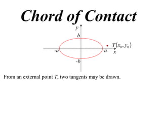
  • 1. Chord of Contact y b T  x0 , y0  -a a x -b From an external point T, two tangents may be drawn.
  • 2. Chord of Contact y b P x1 , y1  T  x0 , y0  -a a x -b From an external point T, two tangents may be drawn. xx yy tangent at P has equation 12  12  1 a b
  • 3. Chord of Contact y b P x1 , y1  T  x0 , y0  -a a x Q  x2 , y 2  -b From an external point T, two tangents may be drawn. xx yy tangent at P has equation 12  12  1 a b xx y y tangent at Q has equation 22  22  1 a b
  • 4. Chord of Contact y b P x1 , y1  T  x0 , y0  -a a x Q  x2 , y 2  -b From an external point T, two tangents may be drawn. xx yy tangent at P has equation 12  12  1 a b xx y y tangent at Q has equation 22  22  1 Now T lies on both lines, a b
  • 5. Chord of Contact y b P x1 , y1  T  x0 , y0  -a a x Q  x2 , y 2  -b From an external point T, two tangents may be drawn. xx yy tangent at P has equation 12  12  1 a b xx y y tangent at Q has equation 22  22  1 Now T lies on both lines, a b xx yy x2 x0 y2 y0  1 2 0  1 2 0  1 and 2  2 1 a b a b
  • 6. y x2 x0 y2 y0 b  2 1 P x1 , y1  a 2 b T  x0 , y0  -a a x Q  x2 , y 2  x1 x0 y1 y0  2 1 2 -b a b Thus P and Q both must lie on a line with equation;
  • 7. y x2 x0 y2 y0 b  2 1 P x1 , y1  a 2 b T  x0 , y0  -a a x Q  x2 , y 2  x1 x0 y1 y0  2 1 2 -b a b Thus P and Q both must lie on a line with equation; x0 x y0 y 2  2 1 a b
  • 8. y x2 x0 y2 y0 b  2 1 P x1 , y1  a 2 b T  x0 , y0  -a a x Q  x2 , y 2  x1 x0 y1 y0  2 1 2 -b a b Thus P and Q both must lie on a line with equation; x0 x y0 y 2  2 1 a b which must be the line PQ i.e. chord of contact
  • 9. y x2 x0 y2 y0 b  2 1 P x1 , y1  a 2 b T  x0 , y0  -a a x Q  x2 , y 2  x1 x0 y1 y0  2 1 2 -b a b Thus P and Q both must lie on a line with equation; x0 x y0 y 2  2 1 a b which must be the line PQ i.e. chord of contact Similarly the chord of contact of the hyperbola has the equation; x0 x y0 y 2  2 1 a b
  • 10. Rectangular Hyperbola y  c P cp,   p  c Q cq,   q x xy  c 2 1) Show that equation PQ is x  pqy  c p  q  (1)
  • 11. Rectangular Hyperbola y  c P cp,   p  c Q cq,  T  x0 , y0   q x xy  c 2 1) Show that equation PQ is x  pqy  c p  q  (1)  2cpq 2c  2) Show that T has coordinates  ,   p  q p  q
  • 12. Rectangular Hyperbola y  c P cp,   p  c Q cq,  T  x0 , y0   q x xy  c 2 1) Show that equation PQ is x  pqy  c p  q  (1)  2cpq 2c  2) Show that T has coordinates  ,   p  q p  q 2cpq 2c  x0  y0  pq pq
  • 13. Rectangular Hyperbola y  c P cp,   p  c Q cq,  T  x0 , y0   q x xy  c 2 1) Show that equation PQ is x  pqy  c p  q  (1)  2cpq 2c  2) Show that T has coordinates  ,   p  q p  q 2cpq 2c  x0  y0  pq pq Substituting into (1); x   p  q x0 y  c p  q  2c
  • 14. Rectangular Hyperbola y  c P cp,   p  c Q cq,  T  x0 , y0   q x xy  c 2 1) Show that equation PQ is x  pqy  c p  q  (1)  2cpq 2c  2) Show that T has coordinates  ,   p  q p  q 2cpq 2c  x0  y0  pq pq Substituting into (1); x   p  q x0 y  c p  q  2c 2cx0 2c 2 x y 2cy0 y0
  • 15. Rectangular Hyperbola y  c P cp,   p  c Q cq,  T  x0 , y0   q x xy  c 2 1) Show that equation PQ is x  pqy  c p  q  (1)  2cpq 2c  2) Show that T has coordinates  ,   p  q p  q 2cpq 2c  x0  y0  pq pq Substituting into (1); x   p  q x0 y  c p  q  2c 2cx0 2c 2 x y xy0  x0 y  2c 2 2cy0 y0
  • 17. Geometric Properties (1) The chord of contact from a point on the directrix is a focal chord.
  • 18. Geometric Properties (1) The chord of contact from a point on the directrix is a focal chord. ellipse  a , y  i.e. x  a As T is on the directrix it has coordinates  0 0  e  e
  • 19. Geometric Properties (1) The chord of contact from a point on the directrix is a focal chord. ellipse  a , y  i.e. x  a As T is on the directrix it has coordinates  0 0  e  e  chord of contact will have the equation; a x   e   yy0  1 a2 b2 x yy0  2 1 ae b
  • 20. Geometric Properties (1) The chord of contact from a point on the directrix is a focal chord. ellipse  a , y  i.e. x  a As T is on the directrix it has coordinates  0 0  e  e  chord of contact will have the equation; a x   e   yy0  1 a2 b2 x yy0  2 1 Substitute in focus (ae,0) ae b
  • 21. Geometric Properties (1) The chord of contact from a point on the directrix is a focal chord. ellipse  a , y  i.e. x  a As T is on the directrix it has coordinates  0 0  e  e  chord of contact will have the equation; a x   e   yy0  1 a2 b2 x yy0  2 1 Substitute in focus (ae,0) ae b ae  0  1 0 ae 1
  • 22. Geometric Properties (1) The chord of contact from a point on the directrix is a focal chord. ellipse As T is on the directrix it has coordinates   a , y  i.e. x  a 0 0  e  e  chord of contact will have the equation; a x   e   yy0  1 a2 b2 x yy0  2 1 Substitute in focus (ae,0) ae b ae  0  1 0  focus lies on chord of contact ae i.e. it is a focal chord 1
  • 23. (2) That part of the tangent between the point of contact and the directrix subtends a right angle at the corresponding focus. y Pa cos , b sin   T S x a x e
  • 24. (2) That part of the tangent between the point of contact and the directrix subtends a right angle at the corresponding focus. y Pa cos , b sin   T Prove: PST  90 S x a x e
  • 25. (2) That part of the tangent between the point of contact and the directrix subtends a right angle at the corresponding focus. y Pa cos , b sin   T Prove: PST  90 S x x cos y sin  equation of tangent is  1 a a a b x cos e a y sin  when x  , e  1 e a b
  • 26. (2) That part of the tangent between the point of contact and the directrix subtends a right angle at the corresponding focus. y Pa cos , b sin   T Prove: PST  90 S x x cos y sin  equation of tangent is  1 a a a b x cos e a y sin  when x  , e  1 e a b cos y sin   1 e b y sin  e  cos  b e be  cos  y e sin 
  • 27. (2) That part of the tangent between the point of contact and the directrix subtends a right angle at the corresponding focus. y Pa cos , b sin   T Prove: PST  90 S x x cos y sin  equation of tangent is  1 a a a b x cos e a y sin  when x  , e  1 e a b cos y sin   1 e b y sin  e  cos a be  cos    T  ,   b e e e sin   be  cos  y e sin 
  • 28. b sin   0 mPS  a cos  ae b sin   acos  e 
  • 29. b sin   0 be  cos  mPS  0 a cos  ae mTS  e sin  b sin  a  ae  acos  e  e be  cos  e   e sin  a  ae 2
  • 30. b sin   0 be  cos  mPS  0 a cos  ae mTS  e sin  b sin  a  ae  acos  e  e be  cos  e   e sin  a  ae 2 be  cos   a 1  e 2 sin 
  • 31. b sin   0 be  cos  mPS  0 a cos  ae mTS  e sin  b sin  a  ae  acos  e  e be  cos  e   e sin  a  ae 2 be  cos   a 1  e 2 sin  be  cos   2 a 1  e 2  sin  a
  • 32. b sin   0 be  cos  mPS  0 a cos  ae mTS  e sin  b sin  a  ae  acos  e  e be  cos  e   e sin  a  ae 2 be  cos   a 1  e 2 sin  be  cos   2 a 1  e 2  sin  a ae  cos   b sin 
  • 33. b sin   0 be  cos  mPS  0 a cos  ae mTS  e sin  b sin  a  ae  acos  e  e be  cos  e   e sin  a  ae 2 be  cos   a 1  e 2 sin  be  cos   2 a 1  e 2  sin  a ae  cos   b sin  b sin  ae  cos  mPS  mTS   acos  e  b sin   1
  • 34. b sin   0 be  cos  mPS  0 a cos  ae mTS  e sin  b sin  a  ae  acos  e  e be  cos  e   e sin  a  ae 2 be  cos   a 1  e 2 sin  be  cos   2 a 1  e 2  sin  a ae  cos   b sin  b sin  ae  cos  mPS  mTS   acos  e  b sin   PST  90  1
  • 35. (3) Reflection Property Tangent to an ellipse at a point P on it is equally inclined to the focal chords through P. T y P T S S x
  • 36. (3) Reflection Property Tangent to an ellipse at a point P on it is equally inclined to the focal chords through P. T y P T S S x Prove: SPT  S PT 
  • 37. (3) Reflection Property Tangent to an ellipse at a point P on it is equally inclined to the focal chords through P. T y P T S S x Prove: SPT  S PT  Construct a line || y axis passing through P
  • 38. (3) Reflection Property Tangent to an ellipse at a point P on it is equally inclined to the focal chords through P. T y P N N T S S x Prove: SPT  S PT  Construct a line || y axis passing through P PT PN  (ratio of intercepts of || lines) PT  PN 
  • 39. (3) Reflection Property Tangent to an ellipse at a point P on it is equally inclined to the focal chords through P. T y P N N T S S x Prove: SPT  S PT  Construct a line || y axis passing through P PT PN  (ratio of intercepts of || lines) PT  PN  PT PT    PN PN 
  • 40. ePN  PS and ePN   PS 
  • 41. ePN  PS and ePN   PS  PT PT    PS PS  e e
  • 42. ePN  PS and ePN   PS  PT PT    PS PS  e e PT PT   PS PS 
  • 43. ePN  PS and ePN   PS  PT PT    PS PS  e e PT PT   PS PS  PST  PS T   90 (proven in property (2))
  • 44. ePN  PS and ePN   PS  PT PT    PS PS  e e PT PT   PS PS  PST  PS T   90 (proven in property (2))  sec SPT  sec S PT 
  • 45. ePN  PS and ePN   PS  PT PT    PS PS  e e PT PT   PS PS  PST  PS T   90 (proven in property (2))  sec SPT  sec S PT  SPT  S PT 
  • 46. ePN  PS and ePN   PS  PT PT    PS PS  e e PT PT   PS PS  PST  PS T   90 (proven in property (2))  sec SPT  sec S PT  SPT  S PT 
  • 47. e.g. Find the cartesian equation of z  2  z  2  8
  • 48. e.g. Find the cartesian equation of z  2  z  2  8 The sum of the focal lengths of an ellipse is constant
  • 49. e.g. Find the cartesian equation of z  2  z  2  8 The sum of the focal lengths of an ellipse is constant 2a  8 a4
  • 50. e.g. Find the cartesian equation of z  2  z  2  8 The sum of the focal lengths of an ellipse is constant 2a  8 ae  2 a4 4e  2 1 e 2
  • 51. e.g. Find the cartesian equation of z  2  z  2  8 The sum of the focal lengths of an ellipse is constant 2a  8 ae  2 b 2  a 2 1  e 2  a4 4e  2  1 b 2  16 1   e 1  4 2  12
  • 52. e.g. Find the cartesian equation of z  2  z  2  8 The sum of the focal lengths of an ellipse is constant 2a  8 ae  2 b 2  a 2 1  e 2  a4 4e  2  1 b 2  16 1   e 1  4 2  12 x2 y2  locus is the ellipse  1 16 12
  • 53. e.g. Find the cartesian equation of z  2  z  2  8 The sum of the focal lengths of an ellipse is constant 2a  8 ae  2 b 2  a 2 1  e 2  a4 4e  2  1 b 2  16 1   e 1  4 2  12 x2 y2  locus is the ellipse  1 16 12 Exercise 6E; 1, 2, 4, 7, 8, 10