
Recomendados
Recomendados
Más contenido relacionado
La actualidad más candente
La actualidad más candente (20)
Destacado
Destacado (10)
Similar a Flood analysis
Similar a Flood analysis (20)
Último
Último (20)
Flood analysis
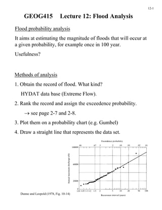
- 1. 12-1 GEOG415 Lecture 12: Flood Analysis Flood probability analysis It aims at estimating the magnitude of floods that will occur at a given probability, for example once in 100 year. Usefulness? Methods of analysis 1. Obtain the record of flood. What kind? HYDAT data base (Extreme Flow). 2. Rank the record and assign the exceedence probability. → see page 2-7 and 2-8. 3. Plot them on a probability chart (e.g. Gumbel) 4. Draw a straight line that represents the data set. Dunne and Leopold (1978, Fig. 10-14)
- 2. 12-2 A map of the areas flooded by the 70-year flood of Bow River. (Montreal Engineering Co., 1973. City of Calgary flood study)
- 3. 12-3 In Fig. 10-14 why does the straight line ignore the highest point? Is it possible that a 100-year flood occurs in a 30-year observation period? How will it show up on the Gumbel plot? Is it OK to estimate 100-year flood from 30-year data by extrapolation? Error estimation Suppose a 30-year annual maximum series having a standard deviation (SD) of 16,000 cfs. The upper bound of the 90 % confidence limit of the 10-year flood is given by (see Table 10-12, next page): SD × 0.50 = 8,000 cfs 8,000 cfs Dunne and Leopold (1978, Fig. 10-17)
- 4. 12-4 Dunne and Leopold (1978, Table 10-12) Every year, there is a 5 % chance of having a 20-year flood . What is the probability of having a 20-year flood in the next five years? → Equation (2-5) in Dunne and Leopold (1978). We have not had a 70-year flood for 71 years. What is the probability of having a 70-year flood next year?
- 5. 12-5 Mean annual flood Gumbel extreme probability distribution is designed so that the average flood (arithmetic mean of all floods in the record) has a theoretical return period of 2.33 years. Using this property, mean annual flood can be determined graphically from a Gumbel chart. Homogeneity of flood records The probability theory commonly used in hydrological analysis assumes that the data are homogeneous. What does it mean? Partial-duration flood series How is it different from annual Dunne and Leopold (1978, Table 10-13) maximum series? What is the actual return period of bankfull discharge?
- 6. 12-6 Regional flood-frequency analysis Planners often require the flood frequency for ungauged basins. → Need for regional frequency curves. Assumption: For large regions of homogeneous climate, vegetation, and topography, individual basins covering a wide range of drainage areas have similar flood-frequency characteristics Dunne and Leopold (1978, Fig. 10-19) Ratio of flood to the mean annual flood 1 1.5 2.33 5 10 25 Dunne and Leopold (1978, Fig. 10-20a) Recurrence interval (years) Floods having specified recurrence interval can be estimated from the mean annual flood.
- 7. 12-7 How is mean annual flood estimated? Is this method applicable in mountainous regions? Dunne and Leopold (1978, Fig. 10-21) Effects of urbanization What are expected effects? tp: lag to peak tp lc: centroid lag lc Dunne and Leopold (1978, Fig. 10-25)
- 8. 12-8 Urban sewer systems reduce centroid lag time. Consequences? S: slope Dunne and Leopold (1978, Fig. 10-26) Dunne and Leopold (1978, Fig. 10-28)
- 9. 12-9 The Unit Hydrograph When the total amount of runoff is given, how do we estimate the temporal distribution of runoff? e.g time lag to peak, duration, etc. The unit hydrograph is the hydrograph of one inch of storm runoff generated by a rainstorm of fairly uniform intensity occurring within a specific period of time (e.g. one hour). The UH theory assumes that temporal distribution depends on basin size, shape, slope, etc., but is fixed from storm to storm. Is this reasonable? Once the UH is established for a basin, hydrographs resulting from any amounts of runoff may be computed from the UH. Hydrograph that would result from 50.8 mm of runoff. 25.4 mm of runoff generated over the basin. Dunne and Leopold (1978, Fig. 10-30)
- 10. 12-10 Construction of the UH from discharge data 1. Select a few storm hydrographs resulting from fairly uniform rain having similar duration, and separate baseflow. 2. Compute the total volume of stormflow (m3) for each hydrograph and divide it by the basin area to obtain total stormflow in depth unit R (mm). 3. Multiply each discharge measurement by 25.4/R so that the total stormflow of the reduced hydrograph is equal to 25.4 mm. 4. Plot the reduced hydrographs and superimpose them, each hydrograph beginning at the same time. 5. By trial and error, draw the unit hydrograph representing the shape of all reduced hydrographs and having a total stormflow of 25.4 mm.
- 11. 12-11 UH’s for storms of various durations Principles of superposition: Four-hour UH consists of the superposition of two two-hour UH. It needs to be divided by a factor of two to adjust for the total stormflow (25.4 mm). Is this reasonable? Under what condition? Dunne and Leopold (1978, Fig. 10-32)
- 12. 12-12 S-curve method Commonly used to derive hydrographs resulting from arbitrary-duration storms. In this example, the original UH was derived for 2.5-hr storm. It is superimposed successively at 2.5-hr interval, resulting in a S- shaped curve. Dunne and Leopold (1978, Fig. 10-33) What does it represent? Two S-curves are now plotted with an offset of 1 hour (a). The difference between the two S-curves represents another hydrograph (b), which is adjusted for the total stormflow to yield the UH of 1-hour storm (c). Dunne and Leopold (1978, Fig. 10-34)
- 13. 12-13 Synthetic UH’s How can we obtain the UH for an ungauged basin? Assumptions? Dunne and Leopold (1978, Fig. 10-35) Snyder method Correlation between the lag to peak (tp, hours) and basin length. tp = Ct (LLc)0.3 L: Length of main stream from outlet to divide (miles) Lc: Distance from the outlet to a point on the stream nearest the centroid of the basin. Ct: Empirical constant (0.3-10) Duration of rainstorm (Dr) and tp were correlated by: Dr = 0.18tp in Snyder’s study. → may not be true in other regions.
- 14. 12-14 The peak discharge (Qpk, ft3 s-1) is given by: Qpk = CpA/tp A: Basin area (mile2) Cp: Empirical constant (370-405) The duration (tb) of the UH could be given by: tb = 72 + 3tp or tb = 5(tp + 0.5Dr) The width of the UH at 75 % (W75, hour) of the peak flow is given by: W75 = 440A/Qpk1.08 Similarly, W50 is given by: W50 = 770A/Qpk1.08 From tp, Dr, tb, Qpk, W75, and W50, the UH can now be synthesized. Dunne and Leopold (1978, Fig. 10-38)
- 15. 12-15 Triangular UH by Soil Conservation Service An alternative method assumes a triangular shape of the UH. The detailed method of construction is given in Dunne and Leopold (1978, p.342-343). In this case, the time of rise to peak (Tr) is given by: Dunne and Leopold (1978, Fig. 10-39) Tr = Dr/2 + tp Dimensionless UH by Soil Conservation Service This method uses dimensionless time (T/Tp) and discharge (Q/Qpk) to plot the UH. Q and T for each basin can be calculated from Fig.10-40 once Tp and Qpk are given. Tp is dependent on the geometry and dimension of the basin. Qpk is dependent on the amount of runoff, which is estimated from the Dunne and Leopold (1978, Fig. 10-40) curve number method.
- 16. 12-16 Both methods by SCS were developed for small agricultural watersheds. Example A 5-km2, reasonably flat watershed has a curve number of 88. Estimated time of concentration (tc, see page 11-14) is 30 minutes. Generate a synthetic hydrograph resulting from 51 mm of rain applied uniformly over a two-hour period. Runoff (R) = 25 mm using the curve number method Tp = 0.5Dr + 0.6tc = 78 min = 1.3 hr from DL, Eq.(10-20) The dimensionless UH is designed so that Qpk ≅ 0.5R/Tp = 0.5 × 25 / 1.3 = 9.6 mm hr-1 In terms of discharge, Qpk = 15.6 mm hr-1 × 5 km2 = 48000 m3 hr-1 = 13 m3 s-1 13 Discharge (m3 s-1) 0 1.3 Time (hour)