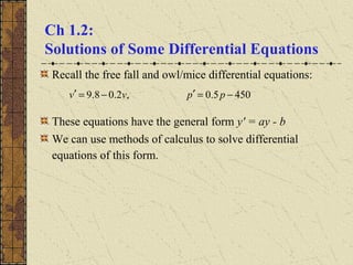
1. Ch 1.2:
Solutions of Some Differential Equations
Recall the free fall and owl/mice differential equations:
These equations have the general form y' = ay - b
We can use methods of calculus to solve differential
equations of this form.
4505.0,2.08.9 −=′−=′ ppvv

2. Example 1: Mice and Owls (1 of 3)
To solve the differential equation
we use methods of calculus, as follows.
Thus the solution is
where k is a constant.
4505.0 −=′ pp
( )
CtCt
Ct
ekkepeep
epCtp
dt
p
dp
p
dtdp
p
dt
dp
±=+=⇒±=−⇒
=−⇒+=−⇒
=
−
⇒=
−
⇒−=
+
∫∫
,900900
9005.0900ln
5.0
900
5.0
900
/
9005.0
5.05.0
5.0
t
kep 5.0
900 +=

3. Example 1: Integral Curves (2 of 3)
Thus we have infinitely many solutions to our equation,
since k is an arbitrary constant.
Graphs of solutions (integral curves) for several values of k,
and direction field for differential equation, are given below.
Choosing k = 0, we obtain the equilibrium solution, while for
k ≠ 0, the solutions diverge from equilibrium solution.
,9004505.0 5.0 t
keppp +=⇒−=′

4. Example 1: Initial Conditions (3 of 3)
A differential equation often has infinitely many solutions. If
a point on the solution curve is known, such as an initial
condition, then this determines a unique solution.
In the mice/owl differential equation, suppose we know that
the mice population starts out at 850. Then p(0) = 850, and
t
t
etp
k
kep
ketp
5.0
0
5.0
50900)(
:Solution
50
900850)0(
900)(
−=
=−
+==
+=

5. Solution to General Equation
To solve the general equation
we use methods of calculus, as follows.
Thus the general solution is
where k is a constant.
bayy −=′
CatCat
Cat
ekkeabyeeaby
eabyCtaaby
dta
aby
dy
a
aby
dtdy
a
b
ya
dt
dy
±=+=⇒±=−⇒
=−⇒+=−⇒
=
−
⇒=
−
⇒





−=
+
∫∫
,//
//ln
//
/
,at
ke
a
b
y +=

6. Initial Value Problem
Next, we solve the initial value problem
From previous slide, the solution to differential equation is
Using the initial condition to solve for k, we obtain
and hence the solution to the initial value problem is
at
e
a
b
y
a
b
y 



−+= 0
0)0(, yybayy =−=′
at
keaby +=
a
b
ykke
a
b
yy −=⇒+== 0
0
0)0(

7. Equilibrium Solution
Recall: To find equilibrium solution, set y' = 0 & solve for y:
From previous slide, our solution to initial value problem is:
Note the following solution behavior:
If y0 = b/a, then y is constant, with y(t) = b/a
If y0 > b/a and a > 0 , then y increases exponentially without bound
If y0 > b/a and a < 0 , then y decays exponentially to b/a
If y0 < b/a and a > 0 , then y decreases exponentially without bound
If y0 < b/a and a < 0 , then y increases asymptotically to b/a
a
b
tybayy
set
=⇒=−=′ )(0
at
e
a
b
y
a
b
y 



−+= 0

8. Example 2: Free Fall Equation (1 of 3)
Recall equation modeling free fall descent of 10 kg object,
assuming an air resistance coefficient γ = 2 kg/sec:
Suppose object is dropped from 300 m. above ground.
(a) Find velocity at any time t.
(b) How long until it hits ground and how fast will it be moving then?
For part (a), we need to solve the initial value problem
Using result from previous slide, we have
0)0(,2.08.9 =−=′ vvv
vdtdv 2.08.9/ −=
( )ttat
eveve
a
b
y
a
b
y 2.2.
0 149
2.0
8.9
0
2.0
8.9 −−
−=⇒



−+=⇒



−+=

9. Example 2: Graphs for Part (a) (2 of 3)
The graph of the solution found in part (a), along with the
direction field for the differential equation, is given below.
( )t
ev
vvv
2.
149
0)0(,2.08.9
−
−=
=−=′

10. Example 2
Part (b): Time and Speed of Impact (3 of 3)
Next, given that the object is dropped from 300 m. above
ground, how long will it take to hit ground, and how fast will
it be moving at impact?
Solution: Let s(t) = distance object has fallen at time t.
It follows from our solution v(t) that
Let T be the time of impact. Then
Using a solver, T ≅ 10.51 sec, hence
24524549)(2450)0(
24549)(4949)()(
2.
2.2.
−+=⇒−=⇒=
++=⇒−==′
−
−−
t
tt
ettsCs
Cettsetvts
30024524549)( 2.
=−+= − T
eTTs
( ) ft/sec01.43149)51.10( )51.10(2.0
≈−= −
ev