SlideShare a Scribd company logo
1 of 14
Download to read offline
Astronomy
&
Astrophysics
A&A 674, A44 (2023)
https://doi.org/10.1051/0004-6361/202345943
© The Authors 2023
Refined parameters of the HD 22946 planetary system
and the true orbital period of planet d⋆,⋆⋆
Z. Garai1,2,3
, H. P. Osborn4,5
, D. Gandolfi6
, A. Brandeker7
, S. G. Sousa8
, M. Lendl12
, A. Bekkelien12
,
C. Broeg4,25
, A. Collier Cameron13
, J. A. Egger4
, M. J. Hooton4,9
, Y. Alibert4
, L. Delrez10,28
, L. Fossati11
,
S. Salmon12
, T. G. Wilson13
, A. Bonfanti14
, A. Tuson9
, S. Ulmer-Moll4,12
, L. M. Serrano6
, L. Borsato15
,
R. Alonso19,29
, G. Anglada20,30
, J. Asquier18
, D. Barrado y Navascues21
, S. C. C. Barros8,24
, T. Bárczy37
,
W. Baumjohann11
, M. Beck12
, T. Beck4
, W. Benz4,25
, N. Billot12
, F. Biondi15,33
, X. Bonfils22
, M. Buder17
,
J. Cabrera17
, V. Cessa4
, S. Charnoz23
, Sz. Csizmadia17
, P. E. Cubillos14,44
, M. B. Davies40
, M. Deleuil31
,
O. D. S. Demangeon22,24
, B.-O. Demory25
, D. Ehrenreich12
, A. Erikson17
, V. Van Eylen45
, A. Fortier4,25
,
M. Fridlund26,27
, M. Gillon10
, V. Van Grootel28
, M. Güdel16
, M. N. Günther18
, S. Hoyer31
, K. G. Isaak18
,
L. L. Kiss38
, M. H. Kristiansen46
, J. Laskar32
, A. Lecavelier des Etangs39
, C. Lovis12
, A. Luntzer16
,
D. Magrin15
, P. F. L. Maxted36
, C. Mordasini4
, V. Nascimbeni15
, G. Olofsson7
, R. Ottensamer16
, I. Pagano35
,
E. Pallé19,29
, G. Peter17
, G. Piotto15,34
, D. Pollacco41
, D. Queloz9,12
, R. Ragazzoni15,34
, N. Rando18
,
H. Rauer17,42
, I. Ribas20,30
, N. C. Santos8,24
, G. Scandariato35
, D. Ségransan12
, A. E. Simon4
,
A. M. S. Smith17
, M. Steller11
, Gy. M. Szabó1,2
, N. Thomas4
, S. Udry12
, J. Venturini12
, and N. Walton43
(Affiliations can be found after the references)
Received 19 January 2023 / Accepted 5 April 2023
ABSTRACT
Context. Multi-planet systems are important sources of information regarding the evolution of planets. However, the long-period
planets in these systems often escape detection. These objects in particular may retain more of their primordial characteristics compared
to close-in counterparts because of their increased distance from the host star. HD 22946 is a bright (G = 8.13 mag) late F-type star
around which three transiting planets were identified via Transiting Exoplanet Survey Satellite (TESS) photometry, but the true orbital
period of the outermost planet d was unknown until now.
Aims. We aim to use the Characterising Exoplanet Satellite (CHEOPS) space telescope to uncover the true orbital period of HD 22946d
and to refine the orbital and planetary properties of the system, especially the radii of the planets.
Methods. We used the available TESS photometry of HD 22946 and observed several transits of the planets b, c, and d using CHEOPS.
We identified two transits of planet d in the TESS photometry, calculated the most probable period aliases based on these data, and
then scheduled CHEOPS observations. The photometric data were supplemented with ESPRESSO (Echelle SPectrograph for Rocky
Exoplanets and Stable Spectroscopic Observations) radial velocity data. Finally, a combined model was fitted to the entire dataset in
order to obtain final planetary and system parameters.
Results. Based on the combined TESS and CHEOPS observations, we successfully determined the true orbital period of the planet d
to be 47.42489 ± 0.00011 days, and derived precise radii of the planets in the system, namely 1.362 ± 0.040 R⊕, 2.328 ± 0.039 R⊕, and
2.607 ± 0.060 R⊕ for planets b, c, and d, respectively. Due to the low number of radial velocities, we were only able to determine 3σ
upper limits for these respective planet masses, which are 13.71 M⊕, 9.72 M⊕, and 26.57 M⊕. We estimated that another 48 ESPRESSO
radial velocities are needed to measure the predicted masses of all planets in HD 22946. We also derived stellar parameters for the host
star.
Conclusions. Planet c around HD 22946 appears to be a promising target for future atmospheric characterisation via transmission
spectroscopy. We can also conclude that planet d, as a warm sub-Neptune, is very interesting because there are only a few similar
confirmed exoplanets to date. Such objects are worth investigating in the near future, for example in terms of their composition and
internal structure.
Key words. methods: observational – techniques: photometric – planets and satellites: fundamental parameters
⋆
Photometry and radial velocity data of HD 22946 are only available at the CDS via anonymous ftp to cdsarc.cds.unistra.fr
(130.79.128.5) or via https://cdsarc.cds.unistra.fr/viz-bin/cat/J/A+A/674/A44
⋆⋆
This article uses data from CHEOPS programmes CH_PR110048 and CH_PR100031.
A44, page 1 of 14
Open Access article, published by EDP Sciences, under the terms of the Creative Commons Attribution License (https://creativecommons.org/licenses/by/4.0),
which permits unrestricted use, distribution, and reproduction in any medium, provided the original work is properly cited.
This article is published in open access under the Subscribe to Open model. Subscribe to A&A to support open access publication.
A&A 674, A44 (2023)
1. Introduction
Multi-planet systems are important from many viewpoints. Not
only are they susceptible of relatively straightforward confir-
mation as bona fide planets (Lissauer et al. 2012), they also
allow intra-planetary comparisons to be made for planets which
formed under the same conditions; see for example Weiss et al.
(2018). The majority of the known multi-planet systems were
found by space-based exoplanet transit surveys. This is because,
while giant hot-Jupiters are relatively easy to observe with
ground-based photometry, the detection of smaller planets, for
example, Earths, super-Earths, and sub-Neptunes, which are
typically found in multi-planet systems, requires the precise
photometry of space-based observatories such as TESS (Ricker
2014).
Mutual gravitational interactions in some multi-planet sys-
tems can provide constraints on the planet masses through
transit time variations (TTVs); see for example Nesvorný &
Morbidelli (2008). Alternatively, radial velocity (RV) observa-
tions are needed to put constraints on the masses of planets
(Mayor & Queloz 1995). Even where masses cannot be deter-
mined, mass upper limits can provide proof that the studied
objects are of planetary origin; see for example Stefánsson et al.
(2020); Hord et al. (2022), or Wilson et al. (2022). Mass determi-
nation can then help constrain the internal structure of the planet
bodies, and break degeneracies in atmospheric characterisation
follow-up studies. If precise planet radii are also determined
from transit photometry, this allows the planet internal density
to be calculated and the planetary composition to be estimated;
see for example Delrez et al. (2021) and Lacedelli et al. (2021,
2022). Precise planetary parameters also allow the planets to
be put in the context of population trends, such as the radius
(Fulton et al. 2017; Van Eylen et al. 2018; Martinez et al. 2019;
Ho & Van Eylen 2023) and density (Luque & Pallé 2022)
valleys.
Long-period planets in multiple-planet systems often escape
detection, especially when their orbital periods are longer than
the typical observing duration of photometric surveys (e.g.
∼27 days for TESS). However, detecting such planets is also
important. For example, the increased distance from their host
stars means that, when compared with close-in planets, they may
retain more of their primordial characteristics, such as unevap-
orated atmospheres (Owen 2019) or circumplanetary material
(Dobos et al. 2021). Due to the limited observing duration of the
TESS primary mission, which observed the majority of the near-
ecliptic sectors for only 27 days, planets on long periods produce
only single transits. However, thanks to its extended mission,
TESS re-observed the same fields 2 yr later, and in many cases
was able to re-detect a second transit; see for example Osborn
et al. (2022). These ‘duotransit’ cases require follow-up in order
to uncover the true orbital period due to the gap, which causes
a set of aliases, P ∈ (ttr,2 − ttr,1)/(1, 2, 3, . . . , Nmax), where ttr,1
and ttr,2 are the first and the second observed mid-transit times,
respectively. The longest possible period is the temporal dis-
tance between the two mid-transit times, Pmax = (ttr,2 − ttr,1), and
the shortest possible period is bounded by the non-detection of
subsequent transits.
In addition to ground-based telescopes, the CHEOPS space
observatory (Benz et al. 2021) can be used to follow-up duo-
transit targets and to determine their true orbital periods and
other characteristics. For example, the periods of two young
sub-Neptunes orbiting BD+40 2790 (TOI-2076, TIC-27491137)
were found using a combination of CHEOPS and ground-based
Table 1. Log of TESS photometric observations of HD 22946.
Time interval of observation Sector no. Transits
HD 22946b
2018-09-20–2018-10-18 03 5
2018-10-18–2018-11-15 04 6
2020-09-22–2020-10-21 30 6
2020-10-21–2020-11-19 31 6
HD 22946c
2018-09-20–2018-10-18 03 2
2018-10-18–2018-11-15 04 2
2020-09-22–2020-10-21 30 2
2020-10-21–2020-11-19 31 2
HD 22946d
2018-10-18–2018-11-15 04 1
2020-09-22–2020-10-21 30 1
photometric follow-up observations (Osborn et al. 2022). Fur-
thermore, these combined observations uncovered the TTVs of
two planets, and also improved the radius precision of all plan-
ets in the system. CHEOPS observations also recovered orbital
periods of duotransits in HIP 9618 (Osborn et al. 2023), TOI-
5678 (Ulmer-Moll et al. 2023), and HD 15906 (Tuson et al. 2023)
systems. In the present study, we investigated the HD 22946 sys-
tem with a similar aim. HD 22946 (TOI-411, TIC-100990000)
is a bright (G = 8.13 mag) late F-type star with three transiting
planets. The planetary system was discovered and validated only
recently by Cacciapuoti et al. (2022, hereafter C22). The authors
presented several parameters of the system, including the radii
and mass limits of the planets. They found that planet b is a
super-Earth with a radius of 1.72±0.10 R⊕, while planets c and d
are sub-Neptunes with radii of 2.74±0.14 R⊕ and 3.23±0.19 R⊕,
respectively. The 3σ upper mass limits of planets b, c, and d
were determined – based on ESPRESSO spectroscopic obser-
vations (see Sect. 2.3) – to be 11 M⊕, 14.5 M⊕, and 24.5 M⊕,
respectively. As TESS recorded several transits during obser-
vations in sector numbers 3, 4, 30, and 31, the discoverers
easily derived the orbital periods of the two inner planets, b
and c, which are about 4040 days and 9573 days, respectively.
The orbital period of planet d was not found by C22. The
authors determined its presence through a single transit found
in sector number 4 and obtained its parameters from this sin-
gle transit event. Its depth and the host brightness make planet d
easily detectable with CHEOPS, and therefore HD 22946 was
observed several times with this instrument within the Guaran-
teed Time Observations (GTO) programmes CH_PR110048 and
CH_PR100031, with the main scientific goals being to uncover
the true orbital period of planet d and to refine the parameters
of the HD 22946 system based on CHEOPS and TESS obser-
vations via joint analysis of the photometric data, supplemented
with ESPRESSO spectroscopic observations of HD 22946.
The present paper is organised as follows. In Sect. 2, we
provide a brief description of observations and data reduction.
In Sect. 3, we present the details of our data analysis and
our first results, including stellar parameters, period aliases of
HD 22946d from the TESS data, and a search for TTVs. Our
final results based on the combined TESS, CHEOPS, and RV
model are described and discussed in Sect. 4. We summarise our
findings in Sect. 5.
A44, page 2 of 14
Garai, Z., et al.: A&A proofs, manuscript no. aa45943-23
Table 2. Log of CHEOPS photometric observations of HD 22946.
Visit Start date End date File CHEOPS Integration Number
No. (UTC) (UTC) key product time (s) of frames
1 2021-10-17 03:22 2021-10-17 14:40 CH_PR100031_TG021201 Subarray 2 × 20.0 629
1 2021-10-17 03:22 2021-10-17 14:40 CH_PR100031_TG021201 Imagettes 20.0 1258
2 2021-10-18 08:14 2021-10-18 19:04 CH_PR100031_TG021101 Subarray 2 × 20.0 637
2 2021-10-18 08:14 2021-10-18 19:04 CH_PR100031_TG021101 Imagettes 20.0 1274
3 2021-10-25 07:08 2021-10-25 19:49 CH_PR110048_TG010001 Subarray 2 × 20.4 708
3 2021-10-25 07:08 2021-10-25 19:49 CH_PR110048_TG010001 Imagettes 20.4 1416
4 2021-10-28 02:12 2021-10-28 13:50 CH_PR110048_TG010101 Subarray 2 × 20.4 666
4 2021-10-28 02:12 2021-10-28 13:50 CH_PR110048_TG010101 Imagettes 20.4 1332
5 2021-10-29 08:48 2021-10-29 18:14 CH_PR100031_TG021202 Subarray 2 × 20.0 555
5 2021-10-29 08:48 2021-10-29 18:14 CH_PR100031_TG021202 Imagettes 20.0 1110
Notes. The time interval of individual observations, the file key, which supports fast identification of the observations in the CHEOPS archive,
type of the photometric product (for more details see Sect. 2.2), the applied integration time, co-added exposures at the subarray type CHEOPS
product, and the number of obtained frames.
2. Observations and data reduction
2.1. TESS data
HD 22946 was observed during four TESS sectors: numbers 3, 4,
30, and 31 (see Table 1). The time gap between the two observ-
ing seasons is almost 2 yr. These TESS data were downloaded
from the Mikulski Archive for Space Telescopes1
in the form
of Presearch Data Conditioning Simple Aperture Photometry
(PDCSAP) flux. These data, containing 61 987 data points, were
obtained from 2-min integrations and were initially smoothed
by the PDCSAP pipeline. This light curve is subjected to more
treatment than the simple aperture photometry (SAP) light curve,
and is specifically intended for detecting planets. The pipeline
attempts to remove systematic artifacts while keeping planetary
transits intact. The average uncertainty of the PDCSAP data
points is 310 ppm.
During these TESS observing runs, 23 transits of planet b
were recorded, and the transit of planet c was observed eight
times in total (see more details in Table 1). As in C22, we also
initially recognised a transit-like feature in the sector number 4
data at ttr,1 = 2 458 425.1657 BJDTDB through visual inspection
of the light curve. Given 65%–80% of single transits from the
TESS primary mission will re-transit in the extended mission
sectors (see Cooke et al. 2019, 2021), we subsequently visually
inspected the light curve once the TESS year 3 data were avail-
able and found a second dip at ttr,2 = 2 459 136.5357 BJDTDB in
the sector number 30 data with near-identical depth and duration.
Given the high prior probability of finding a second transit, the
close match in transit shape between events, and the high quality
of the data (i.e. minimal systematic noise elsewhere in the light
curve), we concluded that this signal is a bona fide transit event
and that the transits in sector numbers 4 and 30 are very likely
caused by the same object, that is, by planet d.
Outliers were cleaned using a 3σ clipping, where σ is the
standard deviation of the light curve. With this clipping pro-
cedure, we discarded 300 data points out of 61 987, which is
∼0.5% of the TESS data. Subsequently, we visually inspected
the dataset in order to check the effect of the outlier removal,
which we found to be reasonable. As TESS uses as time stamps
Barycentric TESS Julian Date (i.e. BJDTDB − 2 457 000.0),
during the next step we converted all TESS time stamps to
BJDTDB.
1 See https://mast.stsci.edu/portal/Mashup/Clients/Mast/
Portal.html
2.2. CHEOPS data
HD 22946 was observed five times with the CHEOPS space
telescope. This is the first European space mission dedicated pri-
marily to the study of known exoplanets. It consists of a telescope
with a mirror of 32 cm in diameter based on a Ritchey-Chrétien
design. The photometric detector is a single-CCD camera cov-
ering the wavelength range from 330 to 1100 nm with a field of
view of 0.32 deg2
. The payload design and operation have been
optimised to achieve ultra-high photometric stability, achieving
a photometric precision of 20 ppm on observations of a G5-type
star in 6 h, and 85 ppm observations of a K5-type star in 3 h
(Benz et al. 2021). The CHEOPS observations were scheduled
based on the existing TESS observations of planets b and c,
and mainly based on the observed transit times of planet d
(see Sect. 2.1). The marginal probability for each period alias
of planet d was calculated using the MonoTools package (see
Sect. 3.2). We were not able to observe all the highest-probability
aliases, because some were not visible during the two-week
period of visibility. Within the program number CH_PR110048,
we therefore planned to observe the three highest-probability
aliases of planet d with CHEOPS, but due to observability con-
straints and conflicts with other observations, only two visits2
of planet d aliases were scheduled. Its true orbital period was
confirmed during the second observation. The remaining three
visits were scheduled in the framework of the program num-
ber CH_PR100031. Based on these CHEOPS observations, three
transits of planet b were recorded during visits 1, 3, and 5, the
transit of planet c was observed twice during visits 2 and 4, and a
single transit of planet d (in multiple transit feature with planet c)
was detected during the CHEOPS visit 4. Further details about
these observations can be found in Table 2.
From the CHEOPS detector, which has 1024 × 1024 pix-
els, a 200 × 200 pixels subarray is extracted around the target
point-spread function (PSF), which is used to compute the pho-
tometry. This type of photometry product was processed by the
CHEOPS Data Reduction Pipeline (DRP) version 13.1.0 (Hoyer
et al. 2020). It performs several image corrections, including
bias-, dark-, and flat-corrections, contamination estimation, and
background-star correction. The DRP pipeline produces four dif-
ferent light-curve types for each visit, but we initially analysed
only the decontaminated ‘OPTIMAL’ type, where the aperture
2 A visit is a sequence of successive CHEOPS orbits devoted to
observing a given target.
A44, page 3 of 14
A&A 674, A44 (2023)
radius is automatically set based on the signal-to-noise ratio
(S/N). In addition to the subarrays, there are imagettes available
for each exposure. The imagettes are frames of 30 pixels in radius
centred on the target, which do not need to be co-added before
download owing to their smaller size. We used a tool specif-
ically developed for photometric extraction of imagettes using
point-spread function photometry, called PIPE3
; see for exam-
ple Szabó et al. (2021, 2022). The PIPE photometry has a S/N
comparable to that of DRP photometry, but has the advantage of
shorter cadence, and therefore we decided to use this CHEOPS
product in this work. The average uncertainty of the PIPE data
points is 160 ppm.
The PIPE CHEOPS observations were processed using the
dedicated data decorrelation and transit analysis software called
pycheops4
(Maxted et al. 2022). This package includes down-
loading, visualising, and decorrelating CHEOPS data, fitting
transits and eclipses of exoplanets, and calculating light-curve
noise. We first cleaned the light curves from outlier data points
using the pycheops built-in function clip_outliers, which
removes outliers from a dataset by calculating the mean absolute
deviation (MAD) from the light curve following median smooth-
ing, and rejects data greater than the smoothed dataset plus the
MAD multiplied by a clipping factor. The clipping factor equal
to five was reasonable in our cases, which we checked visually.
With this clipping procedure, we discarded 30 data points out of
3195, which is ∼0.9% of the CHEOPS data. The next step was
the extraction of the detrending parameters. During this proce-
dure, the software gives a list of the parameters necessary for
the detrending. The most important decorrelation is subtraction
of the roll-angle effect. In order to keep the cold plate radia-
tors facing away from the Earth, the spacecraft rolls during its
orbit. This means that the field of view rotates around the point-
ing direction. The target star remains stationary within typically
1 pixel, but the rotation of the field of view produces a variation
of its flux from the nearby sources in phase with the roll angle
of the spacecraft (Bonfanti et al. 2021). The extracted detrending
parameters were co-fitted with the transit model (see Sect. 3.3).
2.3. ESPRESSO/VLT data
We acquired 14 high-resolution spectra of the host star HD 22946
using the ESPRESSO spectrograph (Pepe et al. 2014) mounted
at the 8.2 m Very Large Telescope (VLT) at Paranal Observatory
(Chile). The observations were carried out between 10 February
2019 and 17 March 2019 under the observing program number
0102.C-0456 (PI: V. Van Eylen) and within the KESPRINT5
project. We used the high-resolution (HR) mode of the spec-
trograph, which provides a resolving power of R ≈ 134 000.
We set the exposure time to 600 s, leading to a S/N per pixel
at 650 nm ranging between 120 and 243. Daytime ThAr spectra
and simultaneous Fabry-Perot exposures were taken to determine
the wavelength solution and correct for possible nightly instru-
mental drifts, respectively. We reduced the ESPRESSO spectra
using the dedicated data-reduction software and extracted the
RVs by cross-correlating the échelle spectra with a G2 numerical
mask. We list the ESPRESSO RV measurements in Table 3. The
average uncertainty of the RV data points is ∼0.00015 km s−1
.
We co-added the individual ESPRESSO spectra prior to
carrying out the spectroscopic analysis presented in Sect. 3.1.
To this aim, we Doppler-shifted the data to a common refer-
ence wavelength by cross-correlating the ESPRESSO spectra
3 See https://github.com/alphapsa/PIPE
4 See https://github.com/pmaxted/pycheops
5 See https://kesprint.science/
Table 3. Log of ESPRESSO/VLT RV observations of HD 22946.
Time (BJDTDB) RV value (km s−1
) ±1σ (km s−1
)
2458524.56069831 16.85125 0.00011
2458525.55490396 16.85217 0.00013
2458526.59541816 16.85512 0.00011
2458527.63233315 16.85284 0.00022
2458535.62345024 16.84839 0.00036
2458540.53620531 16.85020 0.00010
2458550.57174504 16.85549 0.00020
2458552.56783808 16.85330 0.00016
2458553.51738686 16.86251 0.00011
2458556.50131285 16.85536 0.00014
2458557.50492574 16.85738 0.00009
2458557.56483059 16.85716 0.00010
2458558.52709593 16.85741 0.00010
2458559.54006749 16.85690 0.00016
with the spectrum with the highest S/N. We finally performed a
S/N-weighted co-addition of the Doppler-shifted spectra, while
applying a sigma-clipping algorithm to remove possible cosmic-
ray hits and outliers. The co-added spectrum has a S/N of ∼900
per pixel at 650 nm.
3. Data analysis and first results
3.1. Stellar parameters
The spectroscopic stellar parameters (the effective temperature
Teff, the surface gravity log g, the microturbulent velocity vmic,
and the metallicity [Fe/H]; see Table 4) were derived using
the ARES and MOOG codes, following the same methodology as
described in Santos et al. (2013), Sousa (2014), and Sousa et al.
(2021). We used the latest version of the ARES code6
(Sousa et al.
2007, 2015) to measure the equivalent widths of iron lines on the
combined ESPRESSO spectrum. We used a minimisation proce-
dure to find ionisation and excitation equilibrium and converge to
the best set of spectroscopic parameters. This procedure makes
use of a grid of Kurucz model atmospheres (Kurucz 1993a) and
the radiative transfer code MOOG (Sneden 1973).
To derive the radius of the host star HD 22946, we used
a Markov-Chain Monte Carlo (MCMC) modified infrared flux
method. This enables us to calculate the bolometric flux using
stellar atmospheric models defined by our spectral analysis
to build spectral energy distributions (SEDs) that are com-
pared with broadband fluxes and uncertainties from the most
recent data releases for the following bandpasses: Gaia G,
GBP, and GRP, 2MASS J, H, and K, and WISE W1 and W2
(Skrutskie et al. 2006; Wright et al. 2010; Gaia Collaboration
2021). From the bolometric flux, we then determine stellar effec-
tive temperature and angular diameter; this latter is converted
to a radius using the offset-corrected Gaia parallax (Lindegren
et al. 2021). We used Bayesian modeling averaging of the
ATLAS (Kurucz 1993b; Castelli & Kurucz 2003) and PHOENIX
(Allard 2014) catalogues to produce a weighted averaged pos-
terior distribution of the stellar radius in order to account for
uncertainties in stellar atmospheric modelling. We find a value
of Rs = 1.117 ± 0.009 R⊙, which is in 3σ agreement with the
value of 1.157 ± 0.025 R⊙ presented by the discoverers.
We finally determined the stellar mass Ms and stellar
age ts using two different sets of stellar evolutionary models,
6 The last version, ARES v2, can be downloaded at https://github.
com/sousasag/ARES
A44, page 4 of 14
Garai, Z., et al.: A&A proofs, manuscript no. aa45943-23
Table 4. Fundamental parameters of the exoplanet host HD 22946.
Parameter (unit) Value Source
Name HD 22946 –
TOI ID 411 G2021
TIC ID 100990000 S2018
Gaia DR3 ID 4848767461548943104 G2022
RA (J2016) (deg) 54.819528 G2022
Dec (J2016) (deg) −42.76304 G2022
T (TESS) (mag) 7.757 ± 0.006 S2018
G (Gaia) (mag) 8.13 ± 0.69 G2022
J (mag) 7.250 ± 0.027 C2003
H (mag) 7.040 ± 0.044 C2003
K (mag) 6.981 ± 0.029 C2003
Teff (K) 6040 ± 48 C2022
Teff (K) 6169 ± 64 This work
Rs (R⊙) 1.157 ± 0.025 C2022
Rs (R⊙) 1.117 ± 0.009 This work
Ms (M⊙) 1.104 ± 0.012 C2022
Ms (M⊙) 1.098+0.040
−0.039 This work
log g (cgs) 4.26 ± 0.15 C2022
log g (cgs) 4.47 ± 0.11 This work
[Fe/H] (dex) −0.14 ± 0.07 C2022
[Fe/H] (dex) −0.08 ± 0.04 This work
ts (Gyr) 5.0 ± 1.0 C2022
ts (Gyr) 2.5 ± 1.0 This work
vmic (km s−1
) 1.25 ± 0.03 This work
Notes. Abbreviations refer to the following sources: G2021 = Guerrero
et al. (2021), S2018 = Stassun et al. (2018), G2022 = Gaia Collaboration
(2023), C2003 = Cutri et al. (2003), C2022 = Cacciapuoti et al. (2022).
namely PARSEC7
v1.2S (Marigo et al. 2017) and CLES (Code
Liègeois d’Évolution Stellaire), see Scuflaire et al. (2008). More
specifically, we employed the isochrone-placement algorithm
developed by Bonfanti et al. (2015, 2016) to interpolate the input
parameters (Teff, [Fe/H], Rs) within pre-computed grids of PAR-
SEC v1.2S isochrones and tracks to derive a first pair of mass and
age. A second pair of mass and age values, instead, was retrieved
by inputting Teff, [Fe/H], and Rs directly in the CLES code,
which generates the best-fit stellar evolutionary track following
the Levenberg-Marquadt minimisation scheme, as described in
Salmon et al. (2021). After carefully checking the mutual con-
sistency of the two respective pairs of outcomes through the
χ2
-based methodology presented in Bonfanti et al. (2021), we
finally merged (i.e. summed) the two Ms and ts results and
obtained Ms = 1.098 ± 0.040 M⊙ and ts = 2.5 ± 1.0 Gyr. The
mass parameter value of the host star agrees within the uncer-
tainty with the value provided in the discovery paper, which is
1.104 ± 0.012 M⊙. However, the planet host seems to be younger
than previously presented by C22. The discoverers obtained a
value of 5.0 ± 1.0 Gyr. More parameter values, including from
this work, are compared with the discovery-paper parameter
values in Table 4.
3.2. Period aliases of HD 22946d from the TESS data
In order to determine each possible period alias and to schedule
CHEOPS observations of planet d, we first performed a period
analysis of the available TESS data. For this purpose, we used
7 PAdova and TRieste Stellar Evolutionary Code: http://stev.
oapd.inaf.it/cgi-bin/cmd
Table 5. Orbital period aliases of the planet HD 22946d.
Alias Period alias (P) Probability (p)
No. (days) (%)
1 39.5206 17.420
2 41.8454 20.078
3 44.4607 20.341
4 47.4248 18.113
5 50.8122 13.445
6 54.7209 7.061
7 59.2809 2.756
8 64.6701 ∼1.0
Notes. Only the period aliases with a probability of p > 1% are listed
here, as calculated by the MonoTools package from TESS data alone,
i.e. before CHEOPS observations.
the MonoTools package8
(Osborn et al. 2022), which is able to
model transit light curves in case of multiple transits, duotransits,
and monotransits, as well as multiple systems with combina-
tions of such candidates, with both radial velocities and transit
photometry. The package calculates a marginalised probability
distribution across all allowed aliases for a given transit model
by combining priors for each alias. The probabilities are esti-
mated based on two major assumptions, namely that short-period
orbits are highly favoured over long-period ones due to a com-
bination of geometric probability and window function, and that
planets in multi-planet systems have low eccentricities (Kipping
et al. 2013; Van Eylen & Albrecht 2015; Kipping 2018). More
details about this software can be found in Osborn et al. (2022).
The TESS data described in Sect. 2.1 were used during the
fitting procedure using MonoTools. In the case of planet b,
we set as input parameters the reference mid-transit time of
Tc = 2 458 385.7318 BJDTDB, the orbital period of Porb =
4.040330 ± 0.000010 days, the transit duration (transit width)
of W = 3.4 h, and the transit depth of D = 134 ppm. In the
case of planet c, the inputs were Tc = 2 458 386.1878 BJDTDB,
Porb = 9.573117 ± 0.000020 days, W = 3.8 h, and D = 389 ppm.
For planet d, we set as input parameters the two mid-transit times
detected by TESS, namely ttr,1 = 2 458 425.1657 BJDTDB and
ttr,2 = 2 459 136.5357 BJDTDB, the transit duration of W = 6.5 h
and the transit depth of D = 478 ppm. These parameters were
calculated from the TESS data alone.
The orbital period aliases of planet d with a probability of
p > 1% are listed in Table 5. The software MonoTools fore-
casted that a transit of planet d with the orbital period alias
number 2 would take place on 25 October 2021, with a mid-
transit time of Tc = 2 459 513.1441 BJDTDB. This forecasted
event was observed during the third CHEOPS visit (see Table 2),
but the expected transit of planet d did not happen; only the tran-
sit of planet b was recorded that time. After this observation,
we were able to exclude the period alias of P = 41.8454 days
from the list of possible aliases. The next forecast predicted
a transit of planet d on 28 October 2021, with a mid-transit
time of Tc = 2 459 515.9338 BJDTDB, which means that, in
this case, the alias number 4 (see Table 5) was preferred as
its true orbital period. This forecasted event was observed with
CHEOPS during its fourth visit. This time, the transit of planet d
was successfully detected together with a transit of planet c, con-
firming that the period alias of P = 47.4248 days is the true
orbital period of planet d. This result also confirms that the
8 See https://github.com/hposborn/MonoTools
A44, page 5 of 14
A&A 674, A44 (2023)
second transit-like feature of planet d, observed by TESS in sec-
tor number 30, was a real transit event and not an instrumental
artifact as considered by C22. Alternatively, the dip observed at
2 459 136.5357 BJDTDB was a mixture of instrumental effects
and the transit of planet d. With this gathered knowledge about
the true orbital period of planet d, we were able to combine
CHEOPS and TESS photometric observations and RV measure-
ments in order to improve the orbital and planetary parameters
of the HD 22946 system, which were previously obtained only
from the TESS and RV data by the discoverers.
3.3. CHEOPS, TESS, and RV combined model
In order to produce accurate planetary parameters for all three
planets, we built a combined model using all available data, that
is, TESS photometry (described in Sect. 2.1), CHEOPS photom-
etry (described in Sect. 2.2), and ESPRESSO RVs (described
in Sect. 2.3). The combined model was built using the PyMC3
package9
(Salvatier et al. 2016), which performs Hamiltonian
Monte Carlo (HMC) sampling, with Keplerian orbits modeled
with exoplanet package10
(Foreman-Mackey et al. 2021). We
used Gaussian processes (GPs) to model the stellar variability
present in the TESS light curve, opting for a simple harmonic
oscillator (SHO) kernel implemented in the celerite package
(Foreman-Mackey et al. 2017) and a quality factor Q = 1/
√
2, as
is common for quasi-periodic stellar variability. In order to speed
up sampling, we binned the TESS data to 30 min bins far from
transits, keeping 2 min data near transit. As we have reasonable
prior knowledge from theoretical analyses for the expected stellar
limb-darkening (LD) parameters for HD 22946, we used these as
priors in the analysis. We used the quadratic LD law and interpo-
lated tables of coefficients calculated for the TESS (Claret 2018)
and CHEOPS (Claret 2021) passbands using the derived stellar
parameters of Teff = 6169 K and log g = 4.47 (cgs). In order
to guard against systematic errors, we inflated the σ for each
parameter prior to 0.1.
Even though the PIPE light curves for HD 22946 have fewer
systematic features than the DRP light curves, they can still
include flux variations due to the influence of various external
factors. Therefore, we can improve the light curve by decorrelat-
ing the flux data against metadata generated for the instrument
and target. To decipher which decorrelation vectors provide
improvement, we ran an initial PyMC3 model for each CHEOPS
visit using all available ancillary data – sin and cos of rol-
langle, background flux, x and y centroid positions, onboard
temperature and time (which also fits short-timescale stellar vari-
ability). These parameters are normalised to have µ = 0.0 and
σ = 1.0, and decorrelation parameters are given normal priors
with µ = 0.0 and σ set by the root-mean-square (RMS) noise
for each CHEOPS visit. For each visit model, we also included
parameters for any planetary transits present in order to ensure
the transits would not bias the model. After HMC sampling,
we assessed each decorrelation parameter using the average and
standard deviations, keeping only those parameters with a Bayes
Factor of BF > 1. Despite this detrending, shorter-timescale
variation can also be present as a function of roll angle (φ).
Pure detrending against sin and cos of roll angle removes the
largest amplitude systematic trends at low frequencies. These are
those closest in timescale to the transit feature, and so a simpler
detrending technique for such timescales guards against over-
fitting of the transit. However, the CHEOPS light curve typically
9 See https://pypi.org/project/pymc3/
10 See https://pypi.org/project/exoplanet/
also contains systematic noise correlated with roll angle that is
at a lower amplitude and higher frequency. This is not there-
fore adequately removed by simple sin and cos decorrelation.
It is this noise that a more flexible GP is better able to model.
We therefore also included a GP to model the variation of flux
with roll-angle effects. To do this, we first found any potential
large jumps in φ and made sure the time series was continuous
between these jumps (i.e. by moving the zero point and ‘wrap-
ping around’). We then transformed the input data such that it is
continuous in x – by sorting by φ rather than time. Once again,
we used a SHO kernel from celerite with quality factor Q set
at 1/
√
2. As we expected the morphology of the variations to be
preserved for all CHEOPS visits, we used a single shared ker-
nel. We found that the linear decorrelation is the most important,
decreasing the log likelihood by a factor of 1400, but the GP is
responsible for a reduction of a further 450, which means that
use of a GP to model roll-angle flux behaviour is well justified.
As multi-planet systems typically have low eccentricities e
(Van Eylen et al. 2019), and we lack the high number of RVs
capable of resolving any differences in e, we chose to fit only
circular orbits. In order to guard against unphysical negative
values, we used broad log-normal priors for the key transit
and RV amplitude parameters, that is, for Rp/Rs (planet-to-
star radius ratio) and K (RV semi-amplitude). The quantities
derived in Sect. 3.1 are used as priors on the stellar param-
eters in the model. For all datasets – CHEOPS, TESS, and
ESPRESSO –, we included a jitter term using a wide log-normal
prior. We then sampled the combined model using the PyMC_ext
‘sample’ function, which is specifically written for astrophys-
ical applications, and allows us to group independent dataset
parameters (e.g. the CHEOPS visit-specific decorrelation param-
eters) together, thereby speeding up sampling greatly. We used
ten chains, tuning each for 1300 steps before sampling for a
further 1800, resulting in 18 000 unique samples. The sample
have effective sample sizes in the thousands, and the gelmin-
rubin statistics are below 1.01 for all parameters, suggesting they
are sufficiently uncorrelated and unbiased. The full list of fitted
GP hyperparameters and detrending parameters with the corre-
sponding best-fitting values can be found in Appendix A.1. The
best-fitting and derived parameters of the system are described
and discussed in Sect. 4.
3.4. Search for transit-timing variations
In order to look for potential TTVs, we also ran a combined
model using unconstrained timing for each planetary transit
thanks to the TTVorbit function of exoplanet, and an inde-
pendent analysis using the Allesfitter software11
(Günther &
Daylan 2019, 2021), applying a nested sampling fit. Although
C22 already performed such an analysis and found no obvious
sign of TTVs in the system, we repeated this procedure, but in
this case using the CHEOPS data as well. This means mainly that
we included three transits of planet d in the analysis and used a
longer time baseline. We used the same dataset as in Sect. 3.3,
which was co-fitted with a GP using the celerite SHO kernel
in both cases. All planetary and system parameters were fixed as
derived previously, only the GP hyperparameters, the detrending
parameters, and the observed-minus-calculated (O-C) parame-
ters for individual mid-transit times were fitted. Both solutions
are consistent with a linear ephemeris, which means we did not
find any indication of a quadratic trend in the data, in agreement
with the conclusion made by the discoverers. As an illustration,
11 See https://www.allesfitter.com/
A44, page 6 of 14
Garai, Z., et al.: A&A proofs, manuscript no. aa45943-23
Table 6. Best-fitting and derived system and planetary parameters of the HD 22946 planetary system.
Parameter (unit) Description HD 22946b HD 22946c HD 22946d
Tc (BJDTDB) Reference mid-transit time 2 458 385.7321+0.0022
−0.0031 2 459 161.60861+0.00069
−0.00072 2 459 136.53720+0.00087
−0.00083
Porb (days) Orbital period 4.040295+0.000015
−0.000014 9.573083 ± 0.000014 47.42489+0.00010
−0.00011
b Impact parameter 0.21+0.11
−0.13 0.504+0.024
−0.026 0.456+0.026
−0.028
a/Rs Scaled semi-major axis 11.03 ± 0.12 19.61+0.22
−0.23 57.00 ± 0.66
a (au) Semi-major axis 0.05727+0.00085
−0.00082 0.1017+0.0015
−0.0014 0.2958+0.0044
−0.0042
Rp/Rs Planet-to-star radius ratio 0.01119+0.00031
−0.00032 0.01912+0.00026
−0.00027 0.02141+0.00046
−0.00045
tdur (days) Transit duration 0.1281+0.0026
−0.0037 0.1535+0.0015
−0.0014 0.2701+0.0019
−0.0020
Rp (R⊕) planet radius 1.362 ± 0.040 2.328+0.038
−0.039 2.607 ± 0.060
Mp (M⊕) planet mass(⋆)
13.71 9.72 26.57
Mp,est (M⊕) Estimated planet mass(♣)
2.42 ± 0.12 6.04 ± 0.17 7.32 ± 0.28
Mp,est (M⊕) Estimated planet mass(♡)
2.61 ± 0.27(†)
6.61 ± 0.17(‡)
7.90 ± 0.28(‡)
ρp (g cm−3
) planet density(⋆)
18.96 3.15 10.80
K (m s−1
) RV semi-amplitude(⋆)
5.05 2.70 4.31
Ip (W m−2
) Insolation flux 673 884+32 444
−31 606 213 337+10 270
−10 006 25 261+1216
−1184
Tsurf (K) Surface temperature(⋄)
1241 ± 14 931 ± 11 546 ± 6
TSM Transmission spectroscopy metric(♯)
43 ± 4 63 ± 2 43 ± 2
Notes. Based on the joint fit of the TESS and CHEOPS photometric data and RV observations. Table shows the best-fitting value of the given
parameter and its ±1σ uncertainty. The fitted values correspond to quantile 0.50 (median) and the uncertainties to quantils ±0.341 in the parameter
distributions obtained from the samples. (⋆)
Only the 3σ upper limits are listed here due to the low number of the RV observations. (⋄)
Assuming
the albedo value of 0.2. (♣)
Based on the relations presented by Chen & Kipping (2017), assuming that the planet radii are from the interval
of 1.23 < Rp < 14.26 R⊕. (♡)
Based on the relations presented by Otegi et al. (2020). (†)
Assuming that ρp > 3.3 g cm−3
. (‡)
Assuming that ρp <
3.3 g cm−3
. ♯
Based on the criteria set by Kempton et al. (2018), using the scale factor of 1.26, the stellar radius of Rs = 1.117 ± 0.009 R⊙ and
J = 7.250 ± 0.027 mag (see Table 4).
-0.1
-0.05
0
0.05
0.1
1200 1400 1600 1800 2000 2200 2400 2600
O-C
[d]
BJDTDB - 2457000
HD 22946b
HD 22946c
HD 22946d
Fig. 1. Observed-minus-calculated (O-C) diagram of mid-transit times
of the planets HD 22946b, HD 22946c, and HD 22946d obtained using
the Allesfitter package. The O-C values are consistent with a linear
ephemeris, which means no significant TTVs are present in the system.
the obtained O–C diagram of the mid-transit times for planets b,
c, and d from the Allesfitter package is depicted in Fig. 1. We
can see that the O–C values are scattered around O–C = 0.0 d,
which means that no significant TTVs are present in the system.
4. Final results and discussion
The best-fitting and derived parameters from the combined
model are listed in Table 6, and the model posteriors of the
host star are summarised in Appendix A.2. The fitted TESS light
curves from sector numbers 3, 4, 30, and 31 are depicted in the
panels of Figs. 2 and 3. The CHEOPS individual observations
overplotted with the best-fitting models are shown in the panels
of Fig. 4. The RV observations fitted with a spectroscopic orbit
are depicted in Fig. 5.
Here, we present new ephemerides of the planetary orbits,
which we calculated based on the combined model. Thanks to
the combined TESS and CHEOPS observations, we were able
to improve the reference mid-transit times and the orbital peri-
ods of the planets compared to the discovery values. C22 derived
the orbital period parameter values of Porb,b = 4.040301+0.000023
−0.000042
days and Porb,c = 9.573096+0.000026
−0.000023 days, and expected an orbital
period of Porb = 46 ± 4 days for planet d, which was esti-
mated based on the transit duration and depth along with stellar
mass and radius through Kepler’s third law, assuming circular
orbits. We confirmed this prediction, finding an orbital period for
planet d of Porb = 47.42489 ± 0.00011 days. The improved ratios
of the orbital periods are Porb,c/Porb,b = 2.37 and Porb,d/Porb,c =
4.95. Based on the Kepler database, the adjacent planet pairs
in multiple systems show a broad overall peak between period
ratios of 1.5 and 2, followed by a declining tail to larger period
ratios. In addition, there appears to be a sizeable peak just inte-
rior to the period ratio 5 (Steffen & Hwang 2015); therefore, we
can say that the period ratios in HD 22946 fall into statistics and
the seemingly large orbital gap between planets c and d is not
anomalous.
In the combined model, we determined the impact parame-
ter b, which is the projected relative distance of the planet from
the stellar disk centre during the transit midpoint in units of
Rs. Converting these parameter values to the orbit inclination
angle values we can obtain i = 88.90+0.16
−0.05 deg, i = 88.52+0.08
−0.07 deg,
and i = 89.54+0.02
−0.03 deg for planets b, c, and d, respectively. For
comparison, we note that the corresponding discovery values
are ib = 88.3+1.1
−1.2 deg and ic = 88.57+0.86
−0.53 deg. The inclination
A44, page 7 of 14
A&A 674, A44 (2023)
0.999
0.9992
0.9994
0.9996
0.9998
1
1.0002
1.0004
1.0006
1.0008
1.001
1385 1390 1395 1400 1405
Relative
flux
BJDTDB - 2457000
TESS observations - Sector No. 03
Averaged data
Full model
0.999
0.9992
0.9994
0.9996
0.9998
1
1.0002
1.0004
1.0006
1.0008
1.001
1385 1390 1395 1400 1405
Relative
flux
BJDTDB - 2457000
TESS observations - Sector No. 03
Averaged data
Transit model
0.999
0.9992
0.9994
0.9996
0.9998
1
1.0002
1.0004
1.0006
1.0008
1.001
1410 1415 1420 1425 1430 1435
Relative
flux
BJDTDB - 2457000
TESS observations - Sector No. 04
Averaged data
Full model
0.999
0.9992
0.9994
0.9996
0.9998
1
1.0002
1.0004
1.0006
1.0008
1.001
1410 1415 1420 1425 1430 1435
Relative
flux
BJDTDB - 2457000
TESS observations - Sector No. 04
Averaged data
Transit model
0.999
0.9992
0.9994
0.9996
0.9998
1
1.0002
1.0004
1.0006
1.0008
1.001
2115 2120 2125 2130 2135 2140
Relative
flux
BJDTDB - 2457000
TESS observations - Sector No. 30
Averaged data
Full model
0.999
0.9992
0.9994
0.9996
0.9998
1
1.0002
1.0004
1.0006
1.0008
1.001
2115 2120 2125 2130 2135 2140
Relative
flux
BJDTDB - 2457000
TESS observations - Sector No. 30
Averaged data
Transit model
Fig. 2. TESS observations of the transiting planets HD 22946b, HD 22946c, and HD 22946d from sector numbers 3, 4, and 30 overplotted with the
best-fitting model. This model was derived based on the entire CHEOPS and TESS photometric dataset and the RV observations from ESPRESSO
via joint analysis of the data. The left-hand panels show the non-detrended data overplotted with the full model, while the right-hand panels show
the detrended data overplotted with the transit model. We averaged the TESS data for better visualisation of the transit events using a running
average with steps and width of 0.009 and 0.09 day, respectively. We note that an interruption in communications between the instrument and
spacecraft occurred at 2 458 418.54 BJDTDB, resulting in an instrument turn-off until 2 458 421.21 BJDTDB. No data were collected during this
period.
angle of planet d was not determined by C22. According to
the improved parameter values, it seems that only the orbits of
planets b and c are well aligned. planet d is probably not in the
same plane as planets b and c.
Based on the combined TESS and CHEOPS photometry
observations, we redetermined the radii of the planets, which
are 1.362 ± 0.040 R⊕, 2.328 ± 0.039 R⊕, and 2.607 ± 0.060 R⊕
for planets b, c, and d, respectively. The CHEOPS observa-
tions are an added value, because compared to the corresponding
parameter values presented in C22 (Rp,b = 1.72 ± 0.10 R⊕, Rp,c =
2.74 ± 0.14 R⊕, and Rp,d = 3.23 ± 0.19 R⊕), there is a notice-
able improvement in radius precision. Using TESS and CHEOPS
photometry observations, the uncertainties on the planet radius
parameter values were decreased by ∼50%, 68%, and 61% for
A44, page 8 of 14
Garai, Z., et al.: A&A proofs, manuscript no. aa45943-23
0.999
0.9992
0.9994
0.9996
0.9998
1
1.0002
1.0004
1.0006
1.0008
1.001
2145 2150 2155 2160 2165 2170
Relative
flux
BJDTDB - 2457000
TESS observations - Sector No. 31
Averaged data
Full model
0.999
0.9992
0.9994
0.9996
0.9998
1
1.0002
1.0004
1.0006
1.0008
1.001
2145 2150 2155 2160 2165 2170
Relative
flux
BJDTDB - 2457000
TESS observations - Sector No. 31
Averaged data
Transit model
Fig. 3. As in Fig. 2, but for the TESS sector number 31.
planets b, c, and d, respectively. We also note that the parameter
values from this work are in stark contrast to those derived by
C22; these authors found significantly larger radii, that is, larger
by ∼21%, 15%, and 19% for planets b, c, and d, respectively.
We believe this may be due to a misunderstanding of the
LimbDarkLightCurve function in exoplanet. The function
requires the planetary radius Rp in solar radii rather than the
planet-to-star radius ratio Rp/Rs. When misused, the result is an
inflation of Rp/Rs and Rp values by a factor of Rs/R⊕, which
in this case is a factor of about 15%–21%. This mistake can be
seen most clearly in C22, when comparing the models shown in
Fig. 5 with the implied depths in Table 4 (likely derived from
the radius ratio), which are inflated by this factor. Such a mis-
take was also evident during the reanalysis of the BD+40 2790
(TOI-2076) system (Osborn et al. 2022).
According to the radius valley at ∼1.5–2.0 R⊕, which
separates super-Earths and sub-Neptunes (Fulton et al. 2017;
Van Eylen et al. 2018; Martinez et al. 2019; Ho & Van Eylen
2023), and based on the refined planet radii, we find that
planet b is a super-Earth, and planets c and d are similar
in size and are sub-Neptunes, in agreement with C22. It is
well known that small exoplanets have bimodal radius distri-
bution separated by the radius valley. Potential explanations
focus on atmospheric-escape-driven mechanisms, such as photo-
evaporation; see for example Owen (2019). The models showed
that those planets that have radius below 1.5 R⊕ were plan-
ets that initially had hydrogen/helium atmospheres, but ulti-
mately lost them due to atmospheric escape, while those just
above 2.0 R⊕ had hydrogen/helium atmosphere masses of ∼1%
of the core mass. Having HD 22946 planets on either side of
the valley means that planet b could be a photo-evaporated
version of planets c and d. Recently, Luque & Pallé (2022)
presented a brand new approach, arguing that the density of
planets might provide more information than planet radii alone
and proposing that a density gap separates rocky from water-
rich planets. For M dwarf systems, these authors found that
rocky planets form within the ice line while water worlds formed
beyond the ice line and migrated inwards. Given that theoretical
models predict similar results for stars of other types, this sce-
nario could also be possible in the case of the planets orbiting
HD 22946.
Due to the low number of RVs, here we present only
the 3σ upper limits for the planet masses in agreement with
the discoverers. C22 obtained the 3σ upper mass limits of
about 11 M⊕, 14.5 M⊕, and 24.5 M⊕ for planets b, c, and d,
respectively, from the same spectroscopic observations. The 3σ
upper limits for the planet masses from this work are Mp,b =
13.71 M⊕, Mp,c = 9.72 M⊕, and Mp,d = 26.57 M⊕. Similarly
to the discoverers, we obtained very different upper mass lim-
its for planets c and d, although they have similar planet radii,
which could be due to a somewhat different internal structure of
these planets. Applying the relations of Chen & Kipping (2017)
and Otegi et al. (2020), we also re-estimated the planet masses,
which were previously forecasted by the discoverers as 6.29 ±
1.30 M⊕, 7.96 ± 0.69 M⊕, and 10.53 ± 1.05 M⊕ for planets b,
c, and d, respectively. The improved parameter values are pre-
sented in Table 6. Furthermore, taking into account the estimated
planet masses calculated based on the relations of Otegi et al.
(2020), we predicted the number of additional RV measure-
ments required to achieve a 3σ detection on each mass using
the Radial Velocity Follow-up Calculator12
(RVFC; see
Cloutier et al. 2018), and the RV simulator (Wilson et al., in
prep.). Based on these simulations, we obtained that another
27, 24, and 48 ESPRESSO RVs are needed to measure the pre-
dicted masses of planets b, c, and d, respectively. The expected
RV semi-amplitudes assuming the estimated planet masses are
Kb = 1.10 ± 0.12 m s−1
, Kc = 2.08 ± 0.10 m s−1
, and Kd =
1.46 ± 0.08 m s−1
.
C22 also probed the planets from the viewpoint of
future atmospheric characterisation using the transmission spec-
troscopy metric (TSM); see Eq. (1) in Kempton et al. (2018).
The authors obtained the TSM values of 65 ± 10, 89 ± 16, and
67 ± 14 for planets b, c, and d, respectively. We revised these
values based on the results from the present work. The improved
TSM values (see Table 6) do not satisfy the recommended value
of TSM > 90 for planets with a radius of 1.5 < Rp < 10 R⊕. On
the other hand, given that this threshold is set very rigorously, in
agreement with the discoverers, we can note that planet c could
be a feasible target for transmission spectroscopy observations
with future atmospheric characterisation missions, such as the
planned Ariel space observatory (Tinetti et al. 2021).
Finally, we discuss the relevance of planet d among the
known population of similar exoplanets. HD 22946d represents
a warm sub-Neptune. Based on the NASA Exoplanet Archive13
(Akeson et al. 2013), there are 5272 confirmed exoplanets up
to 22 February 2023, but only 63 planets out of 5272 are
12 See http://maestria.astro.umontreal.ca/rvfc/
13 See https://exoplanetarchive.ipac.caltech.edu/index.
html
A44, page 9 of 14
A&A 674, A44 (2023)
0.9992
0.9996
1
1.0004
1.0008
2504.6 2504.7 2504.8 2504.9 2505 2505.1
Relative
flux
1st CHEOPS visit - HD 22946b
Full model
0.9988
0.9992
0.9996
1
1.0004
1.0008
2505.8 2505.9 2506 2506.1 2506.2 2506.3
Relative
flux
BJDTDB - 2457000
2nd CHEOPS visit - HD 22946c
Full model
0.9992
0.9996
1
1.0004
1.0008
2504.6 2504.7 2504.8 2504.9 2505 2505.1
Relative
flux
1st CHEOPS visit - HD 22946b
Transit model
0.9988
0.9992
0.9996
1
1.0004
1.0008
2505.8 2505.9 2506 2506.1 2506.2 2506.3
Relative
flux
BJDTDB - 2457000
2nd CHEOPS visit - HD 22946c
Transit model
0.9992
0.9996
1
1.0004
1.0008
2512.8 2512.9 2513 2513.1 2513.2 2513.3
Relative
flux
3rd CHEOPS visit - HD 22946b
Full model
0.9992
0.9996
1
1.0004
1.0008
2516.9 2517 2517.1 2517.2 2517.3
Relative
flux
BJDTDB - 2457000
5th CHEOPS visit - HD 22946b
Full model
0.9992
0.9996
1
1.0004
1.0008
2512.8 2512.9 2513 2513.1 2513.2 2513.3
Relative
flux
3rd CHEOPS visit - HD 22946b
Transit model
0.9992
0.9996
1
1.0004
1.0008
2516.9 2517 2517.1 2517.2 2517.3
Relative
flux
BJDTDB - 2457000
5th CHEOPS visit - HD 22946b
Transit model
0.9984
0.9988
0.9992
0.9996
1
1.0004
1.0008
2515.6 2515.7 2515.8 2515.9 2516 2516.1
Relative
flux
BJDTDB - 2457000
4th CHEOPS visit - HD 22946c,d
Full model - planet c
Full model - planet d
Full model
0.9984
0.9988
0.9992
0.9996
1
1.0004
1.0008
2515.6 2515.7 2515.8 2515.9 2516 2516.1
Relative
flux
BJDTDB - 2457000
4th CHEOPS visit - HD 22946c,d
Transit model - planet c
Transit model - planet d
Full transit model
Fig. 4. Individual CHEOPS observations of the transiting planets HD 22946b, HD 22946c, and HD 22946d. The observed light curves are overplot-
ted with the best-fitting model. This model was derived based on the entire CHEOPS and TESS photometric dataset and the RV observations from
ESPRESSO via joint analysis of the data. The left-hand panels show the non-detrended data overplotted with the full model, while the right-hand
panels show the detrended data overplotted with the transit model. In the case of the fourth CHEOPS visit, as the multiple transit feature, the
individual transit models of planets c and d are also shown in addition to the summed model.
sub-Neptune sized (1.75 < Rp < 3.5 R⊕) and transiting bright
stars (G ≤ 10 mag). Only 7 planets out of 63 have orbital peri-
ods longer than 30 days and only 4 planets out of 7 have
an equilibrium temperature of below 550 K. Three planets
have a lower insolation flux than planet d, namely TOI-2076d
(Osborn et al. 2022), HD 28109d (Dransfield et al. 2022), and
HD 191939 (Badenas-Agusti et al. 2020). HD 22946d is there-
fore an interesting target for future follow-up observations. One
of the questions to be answered in the near future is the compo-
sition and internal structure of sub-Neptune-type planets. Using
CHEOPS observations, we determined the radius of planet d
with high accuracy. Its true mass could be determined with
another 48 ESPRESSO RV measurements according to the esti-
mate we present above. A combination of mass and radius gives
the overall density, which will be an important step forward
towards understanding sub-Neptunes.
A44, page 10 of 14
Garai, Z., et al.: A&A proofs, manuscript no. aa45943-23
-8
-6
-4
-2
0
2
4
6
8
10
1510 1520 1530 1540 1550 1560 1570
RV
[m/s]
BJDTDB - 2457000
+/-1σ
+/-2σ
Obs. with +/-3σ
RV model
Fig. 5. RV observations taken at ESPRESSO fitted with a spectroscopic
orbit (red line). The 1σ and 2σ uncertainties of the model are plotted
as coloured areas. The uncertainties of the individual RV data points
correspond to a 3σ interval.
5. Conclusions
Based on the combined TESS and CHEOPS observations, we
refined several parameters of the HD 22946 planetary system.
First of all, we improved the ephemerides of the planetary
orbits in comparison with the discovery values. We can confirm
that planets b and c have short orbital periods below 10 days,
namely 4.040295 ± 0.000015 days and 9.573083 ± 0.000014
days, respectively. The third planet, HD 22946d, has an orbital
period of 47.42489 ± 0.00011 days, which we were able to
derive based on additional CHEOPS observations. Furthermore,
based on the combined TESS and CHEOPS observations, we
derived precise radii for the planets, which are 1.362 ± 0.040 R⊕,
2.328 ± 0.039 R⊕, and 2.607 ± 0.060 R⊕ for planets b, c, and d,
respectively. On the one hand, we can confirm the conclusion
of the discoverers that the planetary system consists of a super-
Earth, and planets c and d are sub-Neptunes. On the other hand,
we find the planet radii values to be in tension with the values
presented in the discovery paper, which is very probably due to
misuse of the software by the discoverers. The low number of
ESPRESSO RV measurements allowed us to derive only the 3σ
upper limits for the planet masses, which are 13.71 M⊕, 9.72 M⊕,
and 26.57 M⊕ for planets b, c, and d, respectively.
We also investigated the planets from the viewpoint of
possible future follow-up observations. First of all, we can con-
clude that more RV observations are needed to improve the
planet masses in this system. The applied spectroscopic observa-
tions allowed us to derive precise stellar parameters of the host
star and to fit an initial spectroscopic orbit to the RV data, but
there is ample room for improvement in this way. We estimated
that another 48 ESPRESSO RVs are needed to measure the pre-
dicted masses of all planets in HD 22946. planet c could be a
suitable target for future atmospheric characterisation via trans-
mission spectroscopy. We can also conclude that planet d as a
warm sub-Neptune is very interesting, because there are only
a few similar confirmed exoplanets to date. Thanks to the syn-
ergy of TESS and CHEOPS missions, there is a growing sample
of planets, such as HD 22946d. Such objects are worth inves-
tigating in the near future, for example in order to investigate
their composition and internal structure. Finally, we can mention
that future photometric and/or spectroscopic observations could
also be oriented to searching for further possible planets in this
system.
Acknowledgements. We thank the anonymous reviewer for the helpful comments
and suggestions. CHEOPS is an ESA mission in partnership with Switzerland
with important contributions to the payload and the ground segment from
Austria, Belgium, France, Germany, Hungary, Italy, Portugal, Spain, Sweden,
and the United Kingdom. The CHEOPS Consortium would like to gratefully
acknowledge the support received by all the agencies, offices, universities,
and industries involved. Their flexibility and willingness to explore new
approaches were essential to the success of this mission. This paper includes
data collected with the TESS mission, obtained from the MAST data archive
at the Space Telescope Science Institute (STScI). Funding for the TESS
mission is provided by the NASA Explorer Program. STScI is operated by
the Association of Universities for Research in Astronomy, Inc., under NASA
contract NAS 5-26555. This research has made use of the Exoplanet Follow-up
Observation Program (ExoFOP; DOI: 10.26134/ExoFOP5) website, which is
operated by the California Institute of Technology, under contract with the
National Aeronautics and Space Administration under the Exoplanet Explo-
ration Program. This work has made use of data from the European Space
Agency (ESA) mission Gaia (https://www.cosmos.esa.int/gaia),
processed by the Gaia Data Processing and Analysis Consortium (DPAC,
https://www.cosmos.esa.int/web/gaia/dpac/consortium). Funding
for the DPAC has been provided by national institutions, in particular the insti-
tutions participating in the Gaia Multilateral Agreement. Z.G. acknowledges the
support of the Hungarian National Research, Development and Innovation Office
(NKFIH) grant K-125015, the PRODEX Experiment Agreement No. 4000137122
between the ELTE Eötvös Loránd University and the European Space Agency
(ESA-D/SCI-LE-2021-0025), the VEGA grant of the Slovak Academy of
Sciences No. 2/0031/22, the Slovak Research and Development Agency
contract No. APVV-20-0148, and the support of the city of Szombathely.
Gy.M.Sz. acknowledges the support of the Hungarian National Research,
Development and Innovation Office (NKFIH) grant K-125015, a PRODEX
Institute Agreement between the ELTE Eötvös Loránd University and the
European Space Agency (ESA-D/SCI-LE-2021-0025), the Lendület LP2018-
7/2021 grant of the Hungarian Academy of Science and the support of the city of
Szombathely. A.Br. was supported by the SNSA. A.C.C. acknowledges support
from STFC consolidated grant numbers ST/R000824/1 and ST/V000861/1, and
UKSA grant number ST/R003203/1. B.-O.D. acknowledges support from the
Swiss State Secretariat for Education, Research and Innovation (SERI) under
contract number MB22.00046. This project has received funding from the
European Research Council (ERC) under the European Union’s Horizon 2020
research and innovation programme (project FOUR ACES; grant agreement
No 724427). It has also been carried out in the frame of the National Centre
for Competence in Research PlanetS supported by the Swiss National Science
Foundation (SNSF). D.E. acknowledges financial support from the Swiss
National Science Foundation for project 200021_200726. D.G. gratefully
acknowledges financial support from the CRT foundation under Grant No.
2018.2323 “Gaseousor rocky? Unveiling the nature of small worlds”. This work
was also partially supported by a grant from the Simons Foundation (PI Queloz,
grant number 327127). This work has been carried out within the framework of
the NCCR PlanetS supported by the Swiss National Science Foundation under
grants 51NF40_182901 and 51NF40_205606. I.R.I. acknowledges support from
the Spanish Ministry of Science and Innovation and the European Regional
Development Fund through grant PGC2018-098153-B-C33, as well as the
support of the Generalitat de Catalunya/CERCA programme. This work was
granted access to the HPC resources of MesoPSL financed by the Région
Île-de-France and the project Equip@Meso (reference ANR-10-EQPX-29-01)
of the programme Investissements d’Avenir supervised by the Agence Nationale
pour la Recherche. K.G.I. and M.N.G. are the ESA CHEOPS Project Scientists
and are responsible for the ESA CHEOPS Guest Observers Programme. They
do not participate in, or contribute to, the definition of the Guaranteed Time
Programme of the CHEOPS mission through which observations described
in this paper have been taken, nor to any aspect of target selection for the
programme. The Belgian participation to CHEOPS has been supported by
the Belgian Federal Science Policy Office (BELSPO) in the framework of
the PRODEX Program, and by the University of Liège through an ARC
grant for Concerted Research Actions financed by the Wallonia-Brussels
Federation; L.D. is an F.R.S.-FNRS Postdoctoral Researcher. L.M.S. gratefully
acknowledges financial support from the CRT foundation under Grant No.
2018.2323 “Gaseous or rocky? Unveiling the nature of small worlds”. This
project was supported by the CNES. M.F. and C.M.P. gratefully acknowledge
the support of the Swedish National Space Agency (DNR 65/19, 174/18). M.G.
is an F.R.S.-FNRS Senior Research Associate. M.L. acknowledges support of
the Swiss National Science Foundation under grant number PCEFP2_194576.
N.A.W. acknowledges UKSA grant ST/R004838/1. This work was supported by
FCT – Fundação para a Ciência e a Tecnologia through national funds and by
FEDER through COMPETE2020 – Programa Operacional Competitividade e
Internacionalizacão by these grants: UID/FIS/04434/2019, UIDB/04434/2020,
UIDP/04434/2020, PTDC/FIS-AST/32113/2017 & POCI-01-0145-FEDER-
032113, PTDC/FIS-AST/28953/2017 & POCI-01-0145-FEDER-028953,
A44, page 11 of 14
A&A 674, A44 (2023)
PTDC/FIS-AST/28987/2017 & POCI-01-0145-FEDER-028987, O.D.S.D. is
supported in the form of work contract (DL 57/2016/CP1364/CT0004) funded
by national funds through FCT. P.M. acknowledges support from STFC research
grant number ST/M001040/1. We acknowledge support from the Spanish
Ministry of Science and Innovation and the European Regional Development
Fund through grants ESP2016-80435-C2-1-R, ESP2016-80435-C2-2-R,
PGC2018-098153-B-C33, PGC2018-098153-B-C31, ESP2017-87676-C5-1-R,
MDM-2017-0737 Unidad de Excelencia Maria de Maeztu-Centro de
Astrobiología (INTA-CSIC), as well as the support of the Generalitat de
Catalunya/CERCA programme. The MOC activities have been supported
by the ESA contract No. 4000124370. S.H. gratefully acknowledges CNES
funding through the grant 837319. S.C.C.B. acknowledges support from FCT
through FCT contracts nr. IF/01312/2014/CP1215/CT0004. S.G.S. acknowl-
edges support from FCT through FCT contract no. CEECIND/00826/2018
and POPH/FSE (EC). A.C.C. and T.W. acknowledge support from STFC
consolidated grant numbers ST/R000824/1 and ST/V000861/1, and UKSA
grant number ST/R003203/1. V.V.G. is an F.R.S-FNRS Research Associate.
X.B., S.C., D.G., M.F. and J.L. acknowledge their role as ESA-appointed
CHEOPS science team members. Y.A. and M.J.H. acknowledge the support of
the Swiss National Fund under grant 200020_172746. L.Bo., V.Na., I.Pa., G.Pi.,
R.Ra. and G.Sc. acknowledge support from CHEOPS ASI-INAF agreement n.
2019-29-HH.0. NCS acknowledges support from the European Research Council
through the grant agreement 101052347 (FIERCE). This work was supported
by FCT – Fundação para a Ciência e a Tecnologia through national funds and
by FEDER through COMPETE2020 – Programa Operacional Competitividade
e Internacionalização by these grants: UIDB/04434/2020; UIDP/04434/2020.
A.T. thanks the Science and Technology Facilities Council (STFC) for a PhD
studentship. P.E.C. is funded by the Austrian Science Fund (FWF) Erwin
Schroedinger Fellowship, program J4595-N.
References
Akeson, R. L., Chen, X., Ciardi, D., et al. 2013, PASP, 125, 989
Allard, F. 2014, IAU Symp., 299, 271
Badenas-Agusti, M., Günther, M. N., Daylan, T., et al. 2020, AJ, 160, 113
Benz, W., Broeg, C., Fortier, A., et al. 2021, Exp. Astron., 51, 109
Bonfanti, A., Ortolani, S., Piotto, G., & Nascimbeni, V. 2015, A&A, 575, A18
Bonfanti, A., Ortolani, S., & Nascimbeni, V. 2016, A&A, 585, A5
Bonfanti, A., Delrez, L., Hooton, M. J., et al. 2021, A&A, 646, A157
Cacciapuoti, L., Inno, L., Covone, G., et al. 2022, A&A, 668, A85
Castelli, F., & Kurucz, R. L. 2003, IAU Symp., 210, A20
Chen, J., & Kipping, D. 2017, ApJ, 834, 17
Claret, A. 2018, A&A, 618, A20
Claret, A. 2021, RNAAS, 5, 13
Cloutier, R., Doyon, R., Bouchy, F., & Hébrard, G. 2018, AJ, 156, 82
Cooke, B. F., Pollacco, D., & Bayliss, D. 2019, A&A, 631, A83
Cooke, B. F., Pollacco, D., Anderson, D. R., et al. 2021, MNRAS, 500, 5088
Cutri, R. M., Skrutskie, M. F., van Dyk, S., et al. 2003, VizieR Online Data
Catalog: II/246
Delrez, L., Ehrenreich, D., Alibert, Y., et al. 2021, Nat. Astron., 5, 775
Dobos, V., Charnoz, S., Pál, A., Roque-Bernard, A., & Szabó, G. M. 2021, PASP,
133, 094401
Dransfield, G., Triaud, A. H. M. J., Guillot, T., et al. 2022, MNRAS, 515, 1328
Foreman-Mackey, D., Agol, E., Ambikasaran, S., & Angus, R. 2017, AJ, 154,
220
Foreman-Mackey, D., Luger, R., Agol, E., et al. 2021, J. Open Source Softw., 6,
3285
Fulton, B. J., Petigura, E. A., Howard, A. W., et al. 2017, AJ, 154, 109
Gaia Collaboration (Brown, A. G. A., et al.) 2021, A&A, 649, A1
Gaia Collaboration (Vallenari, A., et al.) 2023, A&A, in press, https://doi.
org/10.1051/0004-6361/202243940
Guerrero, N. M., Seager, S., Huang, C. X., et al. 2021, ApJS, 254, 39
Günther, M. N., & Daylan, T. 2019, Astrophysics Source Code Library [record
ascl:1903.003]
Günther, M. N., & Daylan, T. 2021, ApJS, 254, 13
Ho, C. S. K., & Van Eylen, V. 2023, MNRAS, 519, 4056
Hord, B. J., Colón, K. D., Berger, T. A., et al. 2022, AJ, 164, 13
Hoyer, S., Guterman, P., Demangeon, O., et al. 2020, A&A, 635, A24
Kempton, E. M. R., Bean, J. L., Louie, D. R., et al. 2018, PASP, 130, 114401
Kipping, D. 2018, RNAAS, 2, 223
Kipping, D. M., Spiegel, D. S., & Sasselov, D. D. 2013, MNRAS, 434, 1883
Kurucz, R. L. 1993a, SYNTHE spectrum synthesis programs and line data, CD-
ROM No. 18 (Cambridge, MA: Smithsonian Astrophysical Observatory)
Kurucz, R. L. 1993b, SYNTHE spectrum synthesis programs and line data
(Astrophysics Source Code Library)
Lacedelli, G., Malavolta, L., Borsato, L., et al. 2021, MNRAS, 501, 4148
Lacedelli, G., Wilson, T. G., Malavolta, L., et al. 2022, MNRAS, 511, 4551
Lindegren, L., Bastian, U., Biermann, M., et al. 2021, A&A, 649, A4
Lissauer, J. J., Marcy, G. W., Rowe, J. F., et al. 2012, ApJ, 750, 112
Luque, R., & Pallé, E. 2022, Science, 377, 1211
Marigo, P., Girardi, L., Bressan, A., et al. 2017, ApJ, 835, 77
Martinez, C. F., Cunha, K., Ghezzi, L., & Smith, V. V. 2019, ApJ, 875, 29
Maxted, P. F. L., Ehrenreich, D., Wilson, T. G., et al. 2022, MNRAS, 514,
77
Mayor, M., & Queloz, D. 1995, Nature, 378, 355
Nesvorný, D., & Morbidelli, A. 2008, ApJ, 688, 636
Osborn, H. P., Bonfanti, A., Gandolfi, D., et al. 2022, A&A, 664, A156
Osborn, H. P., Nowak, G., Hébrard, G., et al. 2023, MNRAS, 523, 3069
Otegi, J. F., Bouchy, F., & Helled, R. 2020, A&A, 634, A43
Owen, J. E. 2019, Annu. Rev. Earth Planet. Sci., 47, 67
Pepe, F., Molaro, P., Cristiani, S., et al. 2014, Astron. Nachr., 335, 8
Ricker, G. R. 2014, JAAVSO, 42, 234
Salmon, S. J. A. J., Van Grootel, V., Buldgen, G., Dupret, M. A., & Eggenberger,
P. 2021, A&A, 646, A7
Salvatier, J., Wieckiâ, T. V., & Fonnesbeck, C. 2016, Astrophysics Source Code
Library [record ascl:1610.016]
Santos, N. C., Sousa, S. G., Mortier, A., et al. 2013, A&A, 556, A150
Scuflaire, R., Théado, S., Montalbán, J., et al. 2008, Ap&SS, 316, 83
Skrutskie, M. F., Cutri, R. M., Stiening, R., et al. 2006, AJ, 131, 1163
Sneden, C. A. 1973, Ph.D. Thesis, The University of Texas at Austin, USA
Sousa, S. G. 2014, in Determination of Atmospheric Parameters of B-, A-, Fand
G-Type Stars, eds. E. Niemczura, B. Smalley, & W. Pych (Berlin: Springer),
297
Sousa, S. G., Santos, N. C., Israelian, G., Mayor, M., & Monteiro, M. J. P. F. G.
2007, A&A, 469, 783
Sousa, S. G., Santos, N. C., Adibekyan, V., Delgado-Mena, E., & Israelian, G.
2015, A&A, 577, A67
Sousa, S. G., Adibekyan, V., Delgado-Mena, E., et al. 2021, A&A, 656, A53
Stassun, K. G., Oelkers, R. J., Pepper, J., et al. 2018, AJ, 156, 102
Stefánsson, G., Kopparapu, R., Lin, A., et al. 2020, AJ, 160, 259
Steffen, J. H., & Hwang, J. A. 2015, MNRAS, 448, 1956
Szabó, G. M., Gandolfi, D., Brandeker, A., et al. 2021, A&A, 654, A159
Szabó, G. M., Garai, Z., Brandeker, A., et al. 2022, A&A, 659, A7
Tinetti, G., Eccleston, P., Haswell, C., et al. 2021, ArXiv e-prints
[arXiv:2104.04824]
Tuson, A., Queloz, D., Osborn, H. P., et al. 2023, MNRAS, 523, 3090
Ulmer-Moll, S., Osborn, H. P., Tuson, A., et al. 2023, A&A, 674, A43
Van Eylen, V., & Albrecht, S. 2015, ApJ, 808, 126
Van Eylen, V., Agentoft, C., Lundkvist, M. S., et al. 2018, MNRAS, 479,
4786
Van Eylen, V., Albrecht, S., Huang, X., et al. 2019, AJ, 157, 61
Weiss, L. M., Marcy, G. W., Petigura, E. A., et al. 2018, AJ, 155, 48
Wilson, T. G., Goffo, E., Alibert, Y., et al. 2022, MNRAS, 511, 1043
Wright, E. L., Eisenhardt, P. R. M., Mainzer, A. K., et al. 2010, AJ, 140,
1868
1
MTA-ELTE Exoplanet Research Group, 9700 Szombathely, Szent
Imre h. u. 112, Hungary
e-mail: zgarai@ta3.sk
2
ELTE Gothard Astrophysical Observatory, 9700 Szombathely,
Szent Imre h. u. 112, Hungary
3
Astronomical Institute, Slovak Academy of Sciences, 05960
Tatranská Lomnica, Slovakia
4
Physikalisches Institut, University of Bern, Gesellsschaftstrasse 6,
3012 Bern, Switzerland
5
Department of Physics and Kavli Institute for Astrophysics and
Space Research, Massachusetts Institute of Technology, Cambridge,
MA 02139, USA
6
Dipartimento di Fisica, Universita degli Studi di Torino, via Pietro
Giuria 1, 10125, Torino, Italy
7
Department of Astronomy, Stockholm University, AlbaNova Uni-
versity Center, 10691 Stockholm, Sweden
8
Instituto de Astrofisica e Ciencias do Espaco, Universidade do
Porto, CAUP, Rua das Estrelas, 4150-762 Porto, Portugal
9
Astrophysics Group, Cavendish Laboratory, University of
Cambridge, J.J. Thomson Avenue, Cambridge CB3 0HE, UK
10
Astrobiology Research Unit, Université de Liège, Allée du Six-Août
19C, 4000 Liège, Belgium
11
Space Research Institute, Austrian Academy of Sciences,
Schmiedlstrasse 6, 8042 Graz, Austria
A44, page 12 of 14
Garai, Z., et al.: A&A proofs, manuscript no. aa45943-23
12
Observatoire Astronomique de l’Université de Genève, Chemin
Pegasi 51, Versoix, Switzerland
13
Centre for Exoplanet Science, SUPA School of Physics and Astron-
omy, University of St Andrews, North Haugh, St Andrews KY16
9SS, UK
14
Space Research Institute, Austrian Academy of Sciences,
Schmiedlstrasse 6, 8042 Graz, Austria
15
INAF, Osservatorio Astronomico di Padova, Vicolo
dell’Osservatorio 5, 35122 Padova, Italy
16
Department of Astrophysics, University of Vienna, Tuerkenschanzs-
trasse 17, 1180 Vienna, Austria
17
Institute of Planetary Research, German Aerospace Center (DLR),
Rutherfordstrasse 2, 12489 Berlin, Germany
18
European Space Agency (ESA), European Space Research and
Technology Centre (ESTEC), Keplerlaan 1, 2201 AZ Noordwijk,
The Netherlands
19
Instituto de Astrofisica de Canarias, 38200 La Laguna, Tenerife,
Spain
20
Institut d’Estudis Espacials de Catalunya (IEEC), 08034 Barcelona,
Spain
21
Depto. de Astrofisica, Centro de Astrobiologia (CSIC-INTA), ESAC
campus, 28692 Villanueva de la Cañada (Madrid), Spain
22
Université Grenoble Alpes, CNRS, IPAG, 38000 Grenoble, France
23
Université de Paris, Institut de physique du globe de Paris, CNRS,
75005 Paris, France
24
Departamento de Fisica e Astronomia, Faculdade de Ciencias, Uni-
versidade do Porto, Rua do Campo Alegre, 4169-007 Porto, Portugal
25
Center for Space and Habitability, University of Bern,
Gesellschaftsstrasse 6, 3012 Bern, Switzerland
26
Leiden Observatory, University of Leiden, PO Box 9513, 2300 RA
Leiden, The Netherlands
27
Department of Space, Earth and Environment, Chalmers University
of Technology, Onsala Space Observatory, 43992 Onsala, Sweden
28
Space sciences, Technologies and Astrophysics Research (STAR)
Institute, Université de Liège, 19C Allée du Six-Août, 4000 Liège,
Belgium
29
Departamento de Astrofisica, Universidad de La Laguna, 38206
La Laguna, Tenerife, Spain
30
Institut de Ciencies de l’Espai (ICE, CSIC), Campus UAB, Can
Magrans s/n, 08193 Bellaterra, Spain
31
Aix–Marseille Univ., CNRS, CNES, LAM, 38 rue Frédéric
Joliot-Curie, 13388 Marseille, France
32
IMCCE, UMR8028 CNRS, Observatoire de Paris, PSL Univ.,
Sorbonne Univ., 77 av. Denfert-Rochereau, 75014 Paris, France
33
Max Planck Institute for Extraterrestrial Physics, Giessenbachstrasse
1, 85748 Garching bei München, Germany
34
Dipartimento di Fisica e Astronomia “Galileo Galilei”, Universita
degli Studi di Padova, Vicolo dell’Osservatorio 3, 35122 Padova,
Italy
35
INAF, Osservatorio Astrofisico di Catania, Via S. Sofia 78, 95123
Catania, Italy
36
Astrophysics Group, Keele University, Staffordshire ST5 5BG, UK
37
Admatis, 5. Kandó Kálmán Street, 3534 Miskolc, Hungary
38
Konkoly Observatory, Research Centre for Astronomy and Earth
Sciences, 1121 Budapest, Konkoly Thege Miklós út 15–17, Hungary
39
Institut d’astrophysique de Paris, UMR7095 CNRS, Université
Pierre-et-Marie-Curie, 98bis blvd. Arago, 75014 Paris, France
40
Centre for Mathematical Sciences, Lund University, Box 118, 22100
Lund, Sweden
41
Department of Physics, University of Warwick, Gibbet Hill Road,
Coventry CV4 7AL, UK
42
Center for Astronomy and Astrophysics, Technical University
Berlin, Hardenberstrasse 36, 10623 Berlin, Germany
43
Institute of Astronomy, University of Cambridge, Madingley Road,
Cambridge CB3 0HA, UK
44
INAF, Osservatorio Astrofisico di Torino, Via Osservatorio 20,
10025 Pino Torinese, TO, Italy
45
Department of Space and Climate Physics, Mullard Space Science
Laboratory, Holmbury St Mary RH5 6NT, UK
46
Brorfelde Observatory, Observator Gyldenkernes Vej 7, 4340 Tøl-
løse, Denmark
A44, page 13 of 14
A&A 674, A44 (2023)
Appendix A: Additional tables
Table A.1. Best-fitting GP hyperparameters and detrending parameters.
Parameter [unit] Description Value+1σ
−1σ
log σCHEOPS [ppt] log of scatter in the CHEOPS data −2.384+0.057
−0.061
log σTESS [ppt] log of scatter in the TESS data −2.845+0.024
−0.023
φω0,CHEOPS [1/deg] typical frequency of variation in the shared CHEOPS roll-angle GP 1.70+0.19
−0.16
ω0,TESS [1/d] frequency for the TESS SHOTerm GP kernel 1.87+0.10
−0.09
φS0,CHEOPS scaled power in the shared CHEOPS roll-angle GP 0.0062+0.0010
−0.0009
S 0,TESS scaled power in the TESS SHOTerm GP kernel 0.0066+0.0010
−0.0008
φpower,CHEOPS power in the shared CHEOPS roll-angle GP 0.052+0.020
−0.013
φlengthscale,CHEOPS [deg] typical lengthscale of variation in the shared CHEOPS rollangle GP 3.68+0.38
−0.37
d f/d(time)1st,CHEOPS linear detrending parameter for time trend vs. flux – 1st CHEOPS visit 0.075 ± 0.011
d f/d(bg)1st,CHEOPS linear detrending parameter for background vs. flux – 1st CHEOPS visit −0.026 ± 0.036
d2
f/d(bg)2
1st,CHEOPS quadratic detrending parameter for background vs. flux – 1st CHEOPS visit 0.0278 ± 0.0025
d f/d(centroid x)1st,CHEOPS linear detrending parameter for x centroid vs. flux – 1st CHEOPS visit 0.0386+0.0080
−0.0078
d f/d(centroid y)1st,CHEOPS linear detrending parameter for y centroid vs. flux – 1st CHEOPS visit −0.0458+0.0083
−0.0084
d f/d(centroid x)2nd,CHEOPS linear detrending parameter for x centroid vs. flux – 2nd CHEOPS visit 0.202+0.044
−0.045
d2
f/d(centroid x)2
2nd,CHEOPS quadratic detrending parameter for x centroid vs. flux – 2nd CHEOPS visit −0.0304 ± 0.0083
d f/d(time)3rd,CHEOPS linear detrending parameter for time trend vs. flux – 3rd CHEOPS visit 0.015 ± 0.010
d f/d(centroid y)3rd,CHEOPS linear detrending parameter for y centroid vs. flux – 3rd CHEOPS visit −0.0357+0.0074
−0.0075
d f/d(time)4th,CHEOPS linear detrending parameter for time trend vs. flux – 4th CHEOPS visit 0.103 ± 0.013
d f/d(centroid y)4th,CHEOPS linear detrending parameter for y centroid vs. flux – 4th CHEOPS visit −0.061 ± 0.010
d2
f/d(centroid y)2
4th,CHEOPS quadratic detrending parameter for y centroid vs. flux – 4th CHEOPS visit 0.0086 ± 0.0019
xmean,1st,CHEOPS [ppt] the average offset of the median-normalised flux – 1st CHEOPS visit 0.007 ± 0.011
xmean,2nd,CHEOPS [ppt] the average offset of the median-normalised flux – 2nd CHEOPS visit 0.066 ± 0.011
xmean,3rd,CHEOPS [ppt] the average offset of the median-normalised flux – 3rd CHEOPS visit 0.039 ± 0.010
xmean,4th,CHEOPS [ppt] the average offset of the median-normalised flux – 4th CHEOPS visit 0.314 ± 0.014
xmean,5th,CHEOPS [ppt] the average offset of the median-normalised flux – 5th CHEOPS visit 0.061 ± 0.011
xmean,TESS [ppt] the average offset of the median-normalised flux in TESS data 0.0179+0.0085
−0.0084
Notes. Based on the joint fit of the TESS and CHEOPS photometric data, and RV observations. The table shows the best-fitting value of the given
parameter and its ±1σ uncertainty. The fitted values correspond to quantile 0.50 (median) and the uncertainties to quantils ±0.341 in the parameter
distributions obtained from the samples.
Table A.2. As in Table A.1, but for model posteriors of the host
HD 22946.
Parameter [unit] Description Value+1σ
−1σ
Teff [K] effective temperature 6167+64
−63
log g [cgs] log of surface gravity 4.358 ± 0.016
u1,TESS quadratic LD coefficient 0.196 ± 0.077
u2,TESS quadratic LD coefficient 0.244 ± 0.086
u1,CHEOPS quadratic LD coefficient 0.346+0.081
−0.079
u2,CHEOPS quadratic LD coefficient 0.291+0.089
−0.090
Rs [R⊙] stellar radius 1.1161+0.0088
−0.0089
Ms [M⊙] stellar mass 1.105 ± 0.038
γ [m s−1
] system RV 16 854.48+0.82
−0.76
A44, page 14 of 14

More Related Content

Similar to Refined parameters of the HD 22946 planetary system and the true orbital period of planet d

Evidence for a_spectroscopic_direct_detection_of_reflected_light_from_51_peg_b
Evidence for a_spectroscopic_direct_detection_of_reflected_light_from_51_peg_bEvidence for a_spectroscopic_direct_detection_of_reflected_light_from_51_peg_b
Evidence for a_spectroscopic_direct_detection_of_reflected_light_from_51_peg_bSérgio Sacani
 
An Earth-sized exoplanet with a Mercury-like composition
An Earth-sized exoplanet with a Mercury-like compositionAn Earth-sized exoplanet with a Mercury-like composition
An Earth-sized exoplanet with a Mercury-like compositionSérgio Sacani
 
LHS 475 b: A Venus-sized Planet Orbiting a Nearby M Dwarf
LHS 475 b: A Venus-sized Planet Orbiting a Nearby M DwarfLHS 475 b: A Venus-sized Planet Orbiting a Nearby M Dwarf
LHS 475 b: A Venus-sized Planet Orbiting a Nearby M DwarfSérgio Sacani
 
The kepler 10_planetary_system_revisited_by_harps
The kepler 10_planetary_system_revisited_by_harpsThe kepler 10_planetary_system_revisited_by_harps
The kepler 10_planetary_system_revisited_by_harpsSérgio Sacani
 
The harps n-rocky_planet_search_hd219134b_transiting_rocky_planet
The harps n-rocky_planet_search_hd219134b_transiting_rocky_planetThe harps n-rocky_planet_search_hd219134b_transiting_rocky_planet
The harps n-rocky_planet_search_hd219134b_transiting_rocky_planetSérgio Sacani
 
HD 20329b: An ultra-short-period planet around a solar-type star found by TESS
HD 20329b: An ultra-short-period planet around a solar-type star found by TESSHD 20329b: An ultra-short-period planet around a solar-type star found by TESS
HD 20329b: An ultra-short-period planet around a solar-type star found by TESSSérgio Sacani
 
TESS and CHEOPS discover two warm sub-Neptunes transiting the bright K-dwarf ...
TESS and CHEOPS discover two warm sub-Neptunes transiting the bright K-dwarf ...TESS and CHEOPS discover two warm sub-Neptunes transiting the bright K-dwarf ...
TESS and CHEOPS discover two warm sub-Neptunes transiting the bright K-dwarf ...Sérgio Sacani
 
Hd140283 a star_in_the_solar_neighborhood_that_formed_shortly_after_the_big_bang
Hd140283 a star_in_the_solar_neighborhood_that_formed_shortly_after_the_big_bangHd140283 a star_in_the_solar_neighborhood_that_formed_shortly_after_the_big_bang
Hd140283 a star_in_the_solar_neighborhood_that_formed_shortly_after_the_big_bangSérgio Sacani
 
The Variable Detection of Atmospheric Escape around the Young, Hot Neptune AU...
The Variable Detection of Atmospheric Escape around the Young, Hot Neptune AU...The Variable Detection of Atmospheric Escape around the Young, Hot Neptune AU...
The Variable Detection of Atmospheric Escape around the Young, Hot Neptune AU...Sérgio Sacani
 
Gj 832c a_super_earth_in_the_habitable_zone
Gj 832c a_super_earth_in_the_habitable_zoneGj 832c a_super_earth_in_the_habitable_zone
Gj 832c a_super_earth_in_the_habitable_zoneSérgio Sacani
 
Hubble Space Telescope Observations of NGC 253 Dwarf Satellites: Three Ultra-...
Hubble Space Telescope Observations of NGC 253 Dwarf Satellites: Three Ultra-...Hubble Space Telescope Observations of NGC 253 Dwarf Satellites: Three Ultra-...
Hubble Space Telescope Observations of NGC 253 Dwarf Satellites: Three Ultra-...Sérgio Sacani
 
The Possible Tidal Demise of Kepler’s First Planetary System
The Possible Tidal Demise of Kepler’s First Planetary SystemThe Possible Tidal Demise of Kepler’s First Planetary System
The Possible Tidal Demise of Kepler’s First Planetary SystemSérgio Sacani
 
Discovery of a_probable_4_5_jupiter_mass_exoplanet_to_hd95086_by_direct_imaging
Discovery of a_probable_4_5_jupiter_mass_exoplanet_to_hd95086_by_direct_imagingDiscovery of a_probable_4_5_jupiter_mass_exoplanet_to_hd95086_by_direct_imaging
Discovery of a_probable_4_5_jupiter_mass_exoplanet_to_hd95086_by_direct_imagingSérgio Sacani
 
Seven temperate terrestrial planets around the nearby ultracool dwarf star TR...
Seven temperate terrestrial planets around the nearby ultracool dwarf star TR...Seven temperate terrestrial planets around the nearby ultracool dwarf star TR...
Seven temperate terrestrial planets around the nearby ultracool dwarf star TR...Sérgio Sacani
 
Siena Galaxy Atlas 2020
Siena Galaxy Atlas 2020Siena Galaxy Atlas 2020
Siena Galaxy Atlas 2020Sérgio Sacani
 
The extremely high albedo of LTT 9779 b revealed by CHEOPS
The extremely high albedo of LTT 9779 b revealed by CHEOPSThe extremely high albedo of LTT 9779 b revealed by CHEOPS
The extremely high albedo of LTT 9779 b revealed by CHEOPSSérgio Sacani
 
Kinematics and simulations_of_the_stellar_stream_in_the_halo_of_the_umbrella_...
Kinematics and simulations_of_the_stellar_stream_in_the_halo_of_the_umbrella_...Kinematics and simulations_of_the_stellar_stream_in_the_halo_of_the_umbrella_...
Kinematics and simulations_of_the_stellar_stream_in_the_halo_of_the_umbrella_...Sérgio Sacani
 

Similar to Refined parameters of the HD 22946 planetary system and the true orbital period of planet d (20)

Evidence for a_spectroscopic_direct_detection_of_reflected_light_from_51_peg_b
Evidence for a_spectroscopic_direct_detection_of_reflected_light_from_51_peg_bEvidence for a_spectroscopic_direct_detection_of_reflected_light_from_51_peg_b
Evidence for a_spectroscopic_direct_detection_of_reflected_light_from_51_peg_b
 
An Earth-sized exoplanet with a Mercury-like composition
An Earth-sized exoplanet with a Mercury-like compositionAn Earth-sized exoplanet with a Mercury-like composition
An Earth-sized exoplanet with a Mercury-like composition
 
LHS 475 b: A Venus-sized Planet Orbiting a Nearby M Dwarf
LHS 475 b: A Venus-sized Planet Orbiting a Nearby M DwarfLHS 475 b: A Venus-sized Planet Orbiting a Nearby M Dwarf
LHS 475 b: A Venus-sized Planet Orbiting a Nearby M Dwarf
 
The kepler 10_planetary_system_revisited_by_harps
The kepler 10_planetary_system_revisited_by_harpsThe kepler 10_planetary_system_revisited_by_harps
The kepler 10_planetary_system_revisited_by_harps
 
The harps n-rocky_planet_search_hd219134b_transiting_rocky_planet
The harps n-rocky_planet_search_hd219134b_transiting_rocky_planetThe harps n-rocky_planet_search_hd219134b_transiting_rocky_planet
The harps n-rocky_planet_search_hd219134b_transiting_rocky_planet
 
HD 20329b: An ultra-short-period planet around a solar-type star found by TESS
HD 20329b: An ultra-short-period planet around a solar-type star found by TESSHD 20329b: An ultra-short-period planet around a solar-type star found by TESS
HD 20329b: An ultra-short-period planet around a solar-type star found by TESS
 
TESS and CHEOPS discover two warm sub-Neptunes transiting the bright K-dwarf ...
TESS and CHEOPS discover two warm sub-Neptunes transiting the bright K-dwarf ...TESS and CHEOPS discover two warm sub-Neptunes transiting the bright K-dwarf ...
TESS and CHEOPS discover two warm sub-Neptunes transiting the bright K-dwarf ...
 
Hd140283 a star_in_the_solar_neighborhood_that_formed_shortly_after_the_big_bang
Hd140283 a star_in_the_solar_neighborhood_that_formed_shortly_after_the_big_bangHd140283 a star_in_the_solar_neighborhood_that_formed_shortly_after_the_big_bang
Hd140283 a star_in_the_solar_neighborhood_that_formed_shortly_after_the_big_bang
 
The Variable Detection of Atmospheric Escape around the Young, Hot Neptune AU...
The Variable Detection of Atmospheric Escape around the Young, Hot Neptune AU...The Variable Detection of Atmospheric Escape around the Young, Hot Neptune AU...
The Variable Detection of Atmospheric Escape around the Young, Hot Neptune AU...
 
1803.07867.pdf
1803.07867.pdf1803.07867.pdf
1803.07867.pdf
 
Gj 832c a_super_earth_in_the_habitable_zone
Gj 832c a_super_earth_in_the_habitable_zoneGj 832c a_super_earth_in_the_habitable_zone
Gj 832c a_super_earth_in_the_habitable_zone
 
Hubble Space Telescope Observations of NGC 253 Dwarf Satellites: Three Ultra-...
Hubble Space Telescope Observations of NGC 253 Dwarf Satellites: Three Ultra-...Hubble Space Telescope Observations of NGC 253 Dwarf Satellites: Three Ultra-...
Hubble Space Telescope Observations of NGC 253 Dwarf Satellites: Three Ultra-...
 
The Possible Tidal Demise of Kepler’s First Planetary System
The Possible Tidal Demise of Kepler’s First Planetary SystemThe Possible Tidal Demise of Kepler’s First Planetary System
The Possible Tidal Demise of Kepler’s First Planetary System
 
Discovery of a_probable_4_5_jupiter_mass_exoplanet_to_hd95086_by_direct_imaging
Discovery of a_probable_4_5_jupiter_mass_exoplanet_to_hd95086_by_direct_imagingDiscovery of a_probable_4_5_jupiter_mass_exoplanet_to_hd95086_by_direct_imaging
Discovery of a_probable_4_5_jupiter_mass_exoplanet_to_hd95086_by_direct_imaging
 
Teletransportacion marcikic2003
Teletransportacion  marcikic2003Teletransportacion  marcikic2003
Teletransportacion marcikic2003
 
planets like earth
planets like earthplanets like earth
planets like earth
 
Seven temperate terrestrial planets around the nearby ultracool dwarf star TR...
Seven temperate terrestrial planets around the nearby ultracool dwarf star TR...Seven temperate terrestrial planets around the nearby ultracool dwarf star TR...
Seven temperate terrestrial planets around the nearby ultracool dwarf star TR...
 
Siena Galaxy Atlas 2020
Siena Galaxy Atlas 2020Siena Galaxy Atlas 2020
Siena Galaxy Atlas 2020
 
The extremely high albedo of LTT 9779 b revealed by CHEOPS
The extremely high albedo of LTT 9779 b revealed by CHEOPSThe extremely high albedo of LTT 9779 b revealed by CHEOPS
The extremely high albedo of LTT 9779 b revealed by CHEOPS
 
Kinematics and simulations_of_the_stellar_stream_in_the_halo_of_the_umbrella_...
Kinematics and simulations_of_the_stellar_stream_in_the_halo_of_the_umbrella_...Kinematics and simulations_of_the_stellar_stream_in_the_halo_of_the_umbrella_...
Kinematics and simulations_of_the_stellar_stream_in_the_halo_of_the_umbrella_...
 

More from Sérgio Sacani

Observational constraints on mergers creating magnetism in massive stars
Observational constraints on mergers creating magnetism in massive starsObservational constraints on mergers creating magnetism in massive stars
Observational constraints on mergers creating magnetism in massive starsSérgio Sacani
 
Observation of Gravitational Waves from the Coalescence of a 2.5–4.5 M⊙ Compa...
Observation of Gravitational Waves from the Coalescence of a 2.5–4.5 M⊙ Compa...Observation of Gravitational Waves from the Coalescence of a 2.5–4.5 M⊙ Compa...
Observation of Gravitational Waves from the Coalescence of a 2.5–4.5 M⊙ Compa...Sérgio Sacani
 
The SAMI Galaxy Sur v ey: galaxy spin is more strongly correlated with stella...
The SAMI Galaxy Sur v ey: galaxy spin is more strongly correlated with stella...The SAMI Galaxy Sur v ey: galaxy spin is more strongly correlated with stella...
The SAMI Galaxy Sur v ey: galaxy spin is more strongly correlated with stella...Sérgio Sacani
 
Is Betelgeuse Really Rotating? Synthetic ALMA Observations of Large-scale Con...
Is Betelgeuse Really Rotating? Synthetic ALMA Observations of Large-scale Con...Is Betelgeuse Really Rotating? Synthetic ALMA Observations of Large-scale Con...
Is Betelgeuse Really Rotating? Synthetic ALMA Observations of Large-scale Con...Sérgio Sacani
 
First Direct Imaging of a Kelvin–Helmholtz Instability by PSP/WISPR
First Direct Imaging of a Kelvin–Helmholtz Instability by PSP/WISPRFirst Direct Imaging of a Kelvin–Helmholtz Instability by PSP/WISPR
First Direct Imaging of a Kelvin–Helmholtz Instability by PSP/WISPRSérgio Sacani
 
The Sun’s differential rotation is controlled by high- latitude baroclinicall...
The Sun’s differential rotation is controlled by high- latitude baroclinicall...The Sun’s differential rotation is controlled by high- latitude baroclinicall...
The Sun’s differential rotation is controlled by high- latitude baroclinicall...Sérgio Sacani
 
Hydrogen Column Density Variability in a Sample of Local Compton-Thin AGN
Hydrogen Column Density Variability in a Sample of Local Compton-Thin AGNHydrogen Column Density Variability in a Sample of Local Compton-Thin AGN
Hydrogen Column Density Variability in a Sample of Local Compton-Thin AGNSérgio Sacani
 
Huygens - Exploring Titan A Mysterious World
Huygens - Exploring Titan A Mysterious WorldHuygens - Exploring Titan A Mysterious World
Huygens - Exploring Titan A Mysterious WorldSérgio Sacani
 
The Radcliffe Wave Of Milk Way is oscillating
The Radcliffe Wave Of Milk Way  is oscillatingThe Radcliffe Wave Of Milk Way  is oscillating
The Radcliffe Wave Of Milk Way is oscillatingSérgio Sacani
 
Thermonuclear explosions on neutron stars reveal the speed of their jets
Thermonuclear explosions on neutron stars reveal the speed of their jetsThermonuclear explosions on neutron stars reveal the speed of their jets
Thermonuclear explosions on neutron stars reveal the speed of their jetsSérgio Sacani
 
Identification of Superclusters and Their Properties in the Sloan Digital Sky...
Identification of Superclusters and Their Properties in the Sloan Digital Sky...Identification of Superclusters and Their Properties in the Sloan Digital Sky...
Identification of Superclusters and Their Properties in the Sloan Digital Sky...Sérgio Sacani
 
Digitized Continuous Magnetic Recordings for the August/September 1859 Storms...
Digitized Continuous Magnetic Recordings for the August/September 1859 Storms...Digitized Continuous Magnetic Recordings for the August/September 1859 Storms...
Digitized Continuous Magnetic Recordings for the August/September 1859 Storms...Sérgio Sacani
 
Shiva and Shakti: Presumed Proto-Galactic Fragments in the Inner Milky Way
Shiva and Shakti: Presumed Proto-Galactic Fragments in the Inner Milky WayShiva and Shakti: Presumed Proto-Galactic Fragments in the Inner Milky Way
Shiva and Shakti: Presumed Proto-Galactic Fragments in the Inner Milky WaySérgio Sacani
 
Legacy Analysis of Dark Matter Annihilation from the Milky Way Dwarf Spheroid...
Legacy Analysis of Dark Matter Annihilation from the Milky Way Dwarf Spheroid...Legacy Analysis of Dark Matter Annihilation from the Milky Way Dwarf Spheroid...
Legacy Analysis of Dark Matter Annihilation from the Milky Way Dwarf Spheroid...Sérgio Sacani
 
Introducing the Exoplanet Escape Factor and the Fishbowl Worlds (Two conceptu...
Introducing the Exoplanet Escape Factor and the Fishbowl Worlds (Two conceptu...Introducing the Exoplanet Escape Factor and the Fishbowl Worlds (Two conceptu...
Introducing the Exoplanet Escape Factor and the Fishbowl Worlds (Two conceptu...Sérgio Sacani
 
Revelando Marte - Livro Sobre a Exploração do Planeta Vermelho
Revelando Marte - Livro Sobre a Exploração do Planeta VermelhoRevelando Marte - Livro Sobre a Exploração do Planeta Vermelho
Revelando Marte - Livro Sobre a Exploração do Planeta VermelhoSérgio Sacani
 
Weak-lensing detection of intracluster filaments in the Coma cluster
Weak-lensing detection of intracluster filaments in the Coma clusterWeak-lensing detection of intracluster filaments in the Coma cluster
Weak-lensing detection of intracluster filaments in the Coma clusterSérgio Sacani
 
Quasar and Microquasar Series - Microquasars in our Galaxy
Quasar and Microquasar Series - Microquasars in our GalaxyQuasar and Microquasar Series - Microquasars in our Galaxy
Quasar and Microquasar Series - Microquasars in our GalaxySérgio Sacani
 
A galactic microquasar mimicking winged radio galaxies
A galactic microquasar mimicking winged radio galaxiesA galactic microquasar mimicking winged radio galaxies
A galactic microquasar mimicking winged radio galaxiesSérgio Sacani
 
The Search Of Nine Planet, Pluto (Artigo Histórico)
The Search Of Nine Planet, Pluto (Artigo Histórico)The Search Of Nine Planet, Pluto (Artigo Histórico)
The Search Of Nine Planet, Pluto (Artigo Histórico)Sérgio Sacani
 

More from Sérgio Sacani (20)

Observational constraints on mergers creating magnetism in massive stars
Observational constraints on mergers creating magnetism in massive starsObservational constraints on mergers creating magnetism in massive stars
Observational constraints on mergers creating magnetism in massive stars
 
Observation of Gravitational Waves from the Coalescence of a 2.5–4.5 M⊙ Compa...
Observation of Gravitational Waves from the Coalescence of a 2.5–4.5 M⊙ Compa...Observation of Gravitational Waves from the Coalescence of a 2.5–4.5 M⊙ Compa...
Observation of Gravitational Waves from the Coalescence of a 2.5–4.5 M⊙ Compa...
 
The SAMI Galaxy Sur v ey: galaxy spin is more strongly correlated with stella...
The SAMI Galaxy Sur v ey: galaxy spin is more strongly correlated with stella...The SAMI Galaxy Sur v ey: galaxy spin is more strongly correlated with stella...
The SAMI Galaxy Sur v ey: galaxy spin is more strongly correlated with stella...
 
Is Betelgeuse Really Rotating? Synthetic ALMA Observations of Large-scale Con...
Is Betelgeuse Really Rotating? Synthetic ALMA Observations of Large-scale Con...Is Betelgeuse Really Rotating? Synthetic ALMA Observations of Large-scale Con...
Is Betelgeuse Really Rotating? Synthetic ALMA Observations of Large-scale Con...
 
First Direct Imaging of a Kelvin–Helmholtz Instability by PSP/WISPR
First Direct Imaging of a Kelvin–Helmholtz Instability by PSP/WISPRFirst Direct Imaging of a Kelvin–Helmholtz Instability by PSP/WISPR
First Direct Imaging of a Kelvin–Helmholtz Instability by PSP/WISPR
 
The Sun’s differential rotation is controlled by high- latitude baroclinicall...
The Sun’s differential rotation is controlled by high- latitude baroclinicall...The Sun’s differential rotation is controlled by high- latitude baroclinicall...
The Sun’s differential rotation is controlled by high- latitude baroclinicall...
 
Hydrogen Column Density Variability in a Sample of Local Compton-Thin AGN
Hydrogen Column Density Variability in a Sample of Local Compton-Thin AGNHydrogen Column Density Variability in a Sample of Local Compton-Thin AGN
Hydrogen Column Density Variability in a Sample of Local Compton-Thin AGN
 
Huygens - Exploring Titan A Mysterious World
Huygens - Exploring Titan A Mysterious WorldHuygens - Exploring Titan A Mysterious World
Huygens - Exploring Titan A Mysterious World
 
The Radcliffe Wave Of Milk Way is oscillating
The Radcliffe Wave Of Milk Way  is oscillatingThe Radcliffe Wave Of Milk Way  is oscillating
The Radcliffe Wave Of Milk Way is oscillating
 
Thermonuclear explosions on neutron stars reveal the speed of their jets
Thermonuclear explosions on neutron stars reveal the speed of their jetsThermonuclear explosions on neutron stars reveal the speed of their jets
Thermonuclear explosions on neutron stars reveal the speed of their jets
 
Identification of Superclusters and Their Properties in the Sloan Digital Sky...
Identification of Superclusters and Their Properties in the Sloan Digital Sky...Identification of Superclusters and Their Properties in the Sloan Digital Sky...
Identification of Superclusters and Their Properties in the Sloan Digital Sky...
 
Digitized Continuous Magnetic Recordings for the August/September 1859 Storms...
Digitized Continuous Magnetic Recordings for the August/September 1859 Storms...Digitized Continuous Magnetic Recordings for the August/September 1859 Storms...
Digitized Continuous Magnetic Recordings for the August/September 1859 Storms...
 
Shiva and Shakti: Presumed Proto-Galactic Fragments in the Inner Milky Way
Shiva and Shakti: Presumed Proto-Galactic Fragments in the Inner Milky WayShiva and Shakti: Presumed Proto-Galactic Fragments in the Inner Milky Way
Shiva and Shakti: Presumed Proto-Galactic Fragments in the Inner Milky Way
 
Legacy Analysis of Dark Matter Annihilation from the Milky Way Dwarf Spheroid...
Legacy Analysis of Dark Matter Annihilation from the Milky Way Dwarf Spheroid...Legacy Analysis of Dark Matter Annihilation from the Milky Way Dwarf Spheroid...
Legacy Analysis of Dark Matter Annihilation from the Milky Way Dwarf Spheroid...
 
Introducing the Exoplanet Escape Factor and the Fishbowl Worlds (Two conceptu...
Introducing the Exoplanet Escape Factor and the Fishbowl Worlds (Two conceptu...Introducing the Exoplanet Escape Factor and the Fishbowl Worlds (Two conceptu...
Introducing the Exoplanet Escape Factor and the Fishbowl Worlds (Two conceptu...
 
Revelando Marte - Livro Sobre a Exploração do Planeta Vermelho
Revelando Marte - Livro Sobre a Exploração do Planeta VermelhoRevelando Marte - Livro Sobre a Exploração do Planeta Vermelho
Revelando Marte - Livro Sobre a Exploração do Planeta Vermelho
 
Weak-lensing detection of intracluster filaments in the Coma cluster
Weak-lensing detection of intracluster filaments in the Coma clusterWeak-lensing detection of intracluster filaments in the Coma cluster
Weak-lensing detection of intracluster filaments in the Coma cluster
 
Quasar and Microquasar Series - Microquasars in our Galaxy
Quasar and Microquasar Series - Microquasars in our GalaxyQuasar and Microquasar Series - Microquasars in our Galaxy
Quasar and Microquasar Series - Microquasars in our Galaxy
 
A galactic microquasar mimicking winged radio galaxies
A galactic microquasar mimicking winged radio galaxiesA galactic microquasar mimicking winged radio galaxies
A galactic microquasar mimicking winged radio galaxies
 
The Search Of Nine Planet, Pluto (Artigo Histórico)
The Search Of Nine Planet, Pluto (Artigo Histórico)The Search Of Nine Planet, Pluto (Artigo Histórico)
The Search Of Nine Planet, Pluto (Artigo Histórico)
 

Recently uploaded

Environmental Biotechnology Topic:- Microbial Biosensor
Environmental Biotechnology Topic:- Microbial BiosensorEnvironmental Biotechnology Topic:- Microbial Biosensor
Environmental Biotechnology Topic:- Microbial Biosensorsonawaneprad
 
Microphone- characteristics,carbon microphone, dynamic microphone.pptx
Microphone- characteristics,carbon microphone, dynamic microphone.pptxMicrophone- characteristics,carbon microphone, dynamic microphone.pptx
Microphone- characteristics,carbon microphone, dynamic microphone.pptxpriyankatabhane
 
Microteaching on terms used in filtration .Pharmaceutical Engineering
Microteaching on terms used in filtration .Pharmaceutical EngineeringMicroteaching on terms used in filtration .Pharmaceutical Engineering
Microteaching on terms used in filtration .Pharmaceutical EngineeringPrajakta Shinde
 
Pests of Bengal gram_Identification_Dr.UPR.pdf
Pests of Bengal gram_Identification_Dr.UPR.pdfPests of Bengal gram_Identification_Dr.UPR.pdf
Pests of Bengal gram_Identification_Dr.UPR.pdfPirithiRaju
 
Fertilization: Sperm and the egg—collectively called the gametes—fuse togethe...
Fertilization: Sperm and the egg—collectively called the gametes—fuse togethe...Fertilization: Sperm and the egg—collectively called the gametes—fuse togethe...
Fertilization: Sperm and the egg—collectively called the gametes—fuse togethe...D. B. S. College Kanpur
 
BIOETHICS IN RECOMBINANT DNA TECHNOLOGY.
BIOETHICS IN RECOMBINANT DNA TECHNOLOGY.BIOETHICS IN RECOMBINANT DNA TECHNOLOGY.
BIOETHICS IN RECOMBINANT DNA TECHNOLOGY.PraveenaKalaiselvan1
 
Topic 9- General Principles of International Law.pptx
Topic 9- General Principles of International Law.pptxTopic 9- General Principles of International Law.pptx
Topic 9- General Principles of International Law.pptxJorenAcuavera1
 
Vision and reflection on Mining Software Repositories research in 2024
Vision and reflection on Mining Software Repositories research in 2024Vision and reflection on Mining Software Repositories research in 2024
Vision and reflection on Mining Software Repositories research in 2024AyushiRastogi48
 
Davis plaque method.pptx recombinant DNA technology
Davis plaque method.pptx recombinant DNA technologyDavis plaque method.pptx recombinant DNA technology
Davis plaque method.pptx recombinant DNA technologycaarthichand2003
 
User Guide: Magellan MX™ Weather Station
User Guide: Magellan MX™ Weather StationUser Guide: Magellan MX™ Weather Station
User Guide: Magellan MX™ Weather StationColumbia Weather Systems
 
(9818099198) Call Girls In Noida Sector 14 (NOIDA ESCORTS)
(9818099198) Call Girls In Noida Sector 14 (NOIDA ESCORTS)(9818099198) Call Girls In Noida Sector 14 (NOIDA ESCORTS)
(9818099198) Call Girls In Noida Sector 14 (NOIDA ESCORTS)riyaescorts54
 
Best Call Girls In Sector 29 Gurgaon❤️8860477959 EscorTs Service In 24/7 Delh...
Best Call Girls In Sector 29 Gurgaon❤️8860477959 EscorTs Service In 24/7 Delh...Best Call Girls In Sector 29 Gurgaon❤️8860477959 EscorTs Service In 24/7 Delh...
Best Call Girls In Sector 29 Gurgaon❤️8860477959 EscorTs Service In 24/7 Delh...lizamodels9
 
User Guide: Pulsar™ Weather Station (Columbia Weather Systems)
User Guide: Pulsar™ Weather Station (Columbia Weather Systems)User Guide: Pulsar™ Weather Station (Columbia Weather Systems)
User Guide: Pulsar™ Weather Station (Columbia Weather Systems)Columbia Weather Systems
 
Call Girls in Majnu Ka Tilla Delhi 🔝9711014705🔝 Genuine
Call Girls in Majnu Ka Tilla Delhi 🔝9711014705🔝 GenuineCall Girls in Majnu Ka Tilla Delhi 🔝9711014705🔝 Genuine
Call Girls in Majnu Ka Tilla Delhi 🔝9711014705🔝 Genuinethapagita
 
OECD bibliometric indicators: Selected highlights, April 2024
OECD bibliometric indicators: Selected highlights, April 2024OECD bibliometric indicators: Selected highlights, April 2024
OECD bibliometric indicators: Selected highlights, April 2024innovationoecd
 
STOPPED FLOW METHOD & APPLICATION MURUGAVENI B.pptx
STOPPED FLOW METHOD & APPLICATION MURUGAVENI B.pptxSTOPPED FLOW METHOD & APPLICATION MURUGAVENI B.pptx
STOPPED FLOW METHOD & APPLICATION MURUGAVENI B.pptxMurugaveni B
 
basic entomology with insect anatomy and taxonomy
basic entomology with insect anatomy and taxonomybasic entomology with insect anatomy and taxonomy
basic entomology with insect anatomy and taxonomyDrAnita Sharma
 
Call Girls In Nihal Vihar Delhi ❤️8860477959 Looking Escorts In 24/7 Delhi NCR
Call Girls In Nihal Vihar Delhi ❤️8860477959 Looking Escorts In 24/7 Delhi NCRCall Girls In Nihal Vihar Delhi ❤️8860477959 Looking Escorts In 24/7 Delhi NCR
Call Girls In Nihal Vihar Delhi ❤️8860477959 Looking Escorts In 24/7 Delhi NCRlizamodels9
 
Dubai Calls Girl Lisa O525547819 Lexi Call Girls In Dubai
Dubai Calls Girl Lisa O525547819 Lexi Call Girls In DubaiDubai Calls Girl Lisa O525547819 Lexi Call Girls In Dubai
Dubai Calls Girl Lisa O525547819 Lexi Call Girls In Dubaikojalkojal131
 

Recently uploaded (20)

Environmental Biotechnology Topic:- Microbial Biosensor
Environmental Biotechnology Topic:- Microbial BiosensorEnvironmental Biotechnology Topic:- Microbial Biosensor
Environmental Biotechnology Topic:- Microbial Biosensor
 
Microphone- characteristics,carbon microphone, dynamic microphone.pptx
Microphone- characteristics,carbon microphone, dynamic microphone.pptxMicrophone- characteristics,carbon microphone, dynamic microphone.pptx
Microphone- characteristics,carbon microphone, dynamic microphone.pptx
 
Microteaching on terms used in filtration .Pharmaceutical Engineering
Microteaching on terms used in filtration .Pharmaceutical EngineeringMicroteaching on terms used in filtration .Pharmaceutical Engineering
Microteaching on terms used in filtration .Pharmaceutical Engineering
 
Pests of Bengal gram_Identification_Dr.UPR.pdf
Pests of Bengal gram_Identification_Dr.UPR.pdfPests of Bengal gram_Identification_Dr.UPR.pdf
Pests of Bengal gram_Identification_Dr.UPR.pdf
 
Fertilization: Sperm and the egg—collectively called the gametes—fuse togethe...
Fertilization: Sperm and the egg—collectively called the gametes—fuse togethe...Fertilization: Sperm and the egg—collectively called the gametes—fuse togethe...
Fertilization: Sperm and the egg—collectively called the gametes—fuse togethe...
 
BIOETHICS IN RECOMBINANT DNA TECHNOLOGY.
BIOETHICS IN RECOMBINANT DNA TECHNOLOGY.BIOETHICS IN RECOMBINANT DNA TECHNOLOGY.
BIOETHICS IN RECOMBINANT DNA TECHNOLOGY.
 
Topic 9- General Principles of International Law.pptx
Topic 9- General Principles of International Law.pptxTopic 9- General Principles of International Law.pptx
Topic 9- General Principles of International Law.pptx
 
Vision and reflection on Mining Software Repositories research in 2024
Vision and reflection on Mining Software Repositories research in 2024Vision and reflection on Mining Software Repositories research in 2024
Vision and reflection on Mining Software Repositories research in 2024
 
Davis plaque method.pptx recombinant DNA technology
Davis plaque method.pptx recombinant DNA technologyDavis plaque method.pptx recombinant DNA technology
Davis plaque method.pptx recombinant DNA technology
 
User Guide: Magellan MX™ Weather Station
User Guide: Magellan MX™ Weather StationUser Guide: Magellan MX™ Weather Station
User Guide: Magellan MX™ Weather Station
 
(9818099198) Call Girls In Noida Sector 14 (NOIDA ESCORTS)
(9818099198) Call Girls In Noida Sector 14 (NOIDA ESCORTS)(9818099198) Call Girls In Noida Sector 14 (NOIDA ESCORTS)
(9818099198) Call Girls In Noida Sector 14 (NOIDA ESCORTS)
 
Best Call Girls In Sector 29 Gurgaon❤️8860477959 EscorTs Service In 24/7 Delh...
Best Call Girls In Sector 29 Gurgaon❤️8860477959 EscorTs Service In 24/7 Delh...Best Call Girls In Sector 29 Gurgaon❤️8860477959 EscorTs Service In 24/7 Delh...
Best Call Girls In Sector 29 Gurgaon❤️8860477959 EscorTs Service In 24/7 Delh...
 
Volatile Oils Pharmacognosy And Phytochemistry -I
Volatile Oils Pharmacognosy And Phytochemistry -IVolatile Oils Pharmacognosy And Phytochemistry -I
Volatile Oils Pharmacognosy And Phytochemistry -I
 
User Guide: Pulsar™ Weather Station (Columbia Weather Systems)
User Guide: Pulsar™ Weather Station (Columbia Weather Systems)User Guide: Pulsar™ Weather Station (Columbia Weather Systems)
User Guide: Pulsar™ Weather Station (Columbia Weather Systems)
 
Call Girls in Majnu Ka Tilla Delhi 🔝9711014705🔝 Genuine
Call Girls in Majnu Ka Tilla Delhi 🔝9711014705🔝 GenuineCall Girls in Majnu Ka Tilla Delhi 🔝9711014705🔝 Genuine
Call Girls in Majnu Ka Tilla Delhi 🔝9711014705🔝 Genuine
 
OECD bibliometric indicators: Selected highlights, April 2024
OECD bibliometric indicators: Selected highlights, April 2024OECD bibliometric indicators: Selected highlights, April 2024
OECD bibliometric indicators: Selected highlights, April 2024
 
STOPPED FLOW METHOD & APPLICATION MURUGAVENI B.pptx
STOPPED FLOW METHOD & APPLICATION MURUGAVENI B.pptxSTOPPED FLOW METHOD & APPLICATION MURUGAVENI B.pptx
STOPPED FLOW METHOD & APPLICATION MURUGAVENI B.pptx
 
basic entomology with insect anatomy and taxonomy
basic entomology with insect anatomy and taxonomybasic entomology with insect anatomy and taxonomy
basic entomology with insect anatomy and taxonomy
 
Call Girls In Nihal Vihar Delhi ❤️8860477959 Looking Escorts In 24/7 Delhi NCR
Call Girls In Nihal Vihar Delhi ❤️8860477959 Looking Escorts In 24/7 Delhi NCRCall Girls In Nihal Vihar Delhi ❤️8860477959 Looking Escorts In 24/7 Delhi NCR
Call Girls In Nihal Vihar Delhi ❤️8860477959 Looking Escorts In 24/7 Delhi NCR
 
Dubai Calls Girl Lisa O525547819 Lexi Call Girls In Dubai
Dubai Calls Girl Lisa O525547819 Lexi Call Girls In DubaiDubai Calls Girl Lisa O525547819 Lexi Call Girls In Dubai
Dubai Calls Girl Lisa O525547819 Lexi Call Girls In Dubai
 

Refined parameters of the HD 22946 planetary system and the true orbital period of planet d

  • 1. Astronomy & Astrophysics A&A 674, A44 (2023) https://doi.org/10.1051/0004-6361/202345943 © The Authors 2023 Refined parameters of the HD 22946 planetary system and the true orbital period of planet d⋆,⋆⋆ Z. Garai1,2,3 , H. P. Osborn4,5 , D. Gandolfi6 , A. Brandeker7 , S. G. Sousa8 , M. Lendl12 , A. Bekkelien12 , C. Broeg4,25 , A. Collier Cameron13 , J. A. Egger4 , M. J. Hooton4,9 , Y. Alibert4 , L. Delrez10,28 , L. Fossati11 , S. Salmon12 , T. G. Wilson13 , A. Bonfanti14 , A. Tuson9 , S. Ulmer-Moll4,12 , L. M. Serrano6 , L. Borsato15 , R. Alonso19,29 , G. Anglada20,30 , J. Asquier18 , D. Barrado y Navascues21 , S. C. C. Barros8,24 , T. Bárczy37 , W. Baumjohann11 , M. Beck12 , T. Beck4 , W. Benz4,25 , N. Billot12 , F. Biondi15,33 , X. Bonfils22 , M. Buder17 , J. Cabrera17 , V. Cessa4 , S. Charnoz23 , Sz. Csizmadia17 , P. E. Cubillos14,44 , M. B. Davies40 , M. Deleuil31 , O. D. S. Demangeon22,24 , B.-O. Demory25 , D. Ehrenreich12 , A. Erikson17 , V. Van Eylen45 , A. Fortier4,25 , M. Fridlund26,27 , M. Gillon10 , V. Van Grootel28 , M. Güdel16 , M. N. Günther18 , S. Hoyer31 , K. G. Isaak18 , L. L. Kiss38 , M. H. Kristiansen46 , J. Laskar32 , A. Lecavelier des Etangs39 , C. Lovis12 , A. Luntzer16 , D. Magrin15 , P. F. L. Maxted36 , C. Mordasini4 , V. Nascimbeni15 , G. Olofsson7 , R. Ottensamer16 , I. Pagano35 , E. Pallé19,29 , G. Peter17 , G. Piotto15,34 , D. Pollacco41 , D. Queloz9,12 , R. Ragazzoni15,34 , N. Rando18 , H. Rauer17,42 , I. Ribas20,30 , N. C. Santos8,24 , G. Scandariato35 , D. Ségransan12 , A. E. Simon4 , A. M. S. Smith17 , M. Steller11 , Gy. M. Szabó1,2 , N. Thomas4 , S. Udry12 , J. Venturini12 , and N. Walton43 (Affiliations can be found after the references) Received 19 January 2023 / Accepted 5 April 2023 ABSTRACT Context. Multi-planet systems are important sources of information regarding the evolution of planets. However, the long-period planets in these systems often escape detection. These objects in particular may retain more of their primordial characteristics compared to close-in counterparts because of their increased distance from the host star. HD 22946 is a bright (G = 8.13 mag) late F-type star around which three transiting planets were identified via Transiting Exoplanet Survey Satellite (TESS) photometry, but the true orbital period of the outermost planet d was unknown until now. Aims. We aim to use the Characterising Exoplanet Satellite (CHEOPS) space telescope to uncover the true orbital period of HD 22946d and to refine the orbital and planetary properties of the system, especially the radii of the planets. Methods. We used the available TESS photometry of HD 22946 and observed several transits of the planets b, c, and d using CHEOPS. We identified two transits of planet d in the TESS photometry, calculated the most probable period aliases based on these data, and then scheduled CHEOPS observations. The photometric data were supplemented with ESPRESSO (Echelle SPectrograph for Rocky Exoplanets and Stable Spectroscopic Observations) radial velocity data. Finally, a combined model was fitted to the entire dataset in order to obtain final planetary and system parameters. Results. Based on the combined TESS and CHEOPS observations, we successfully determined the true orbital period of the planet d to be 47.42489 ± 0.00011 days, and derived precise radii of the planets in the system, namely 1.362 ± 0.040 R⊕, 2.328 ± 0.039 R⊕, and 2.607 ± 0.060 R⊕ for planets b, c, and d, respectively. Due to the low number of radial velocities, we were only able to determine 3σ upper limits for these respective planet masses, which are 13.71 M⊕, 9.72 M⊕, and 26.57 M⊕. We estimated that another 48 ESPRESSO radial velocities are needed to measure the predicted masses of all planets in HD 22946. We also derived stellar parameters for the host star. Conclusions. Planet c around HD 22946 appears to be a promising target for future atmospheric characterisation via transmission spectroscopy. We can also conclude that planet d, as a warm sub-Neptune, is very interesting because there are only a few similar confirmed exoplanets to date. Such objects are worth investigating in the near future, for example in terms of their composition and internal structure. Key words. methods: observational – techniques: photometric – planets and satellites: fundamental parameters ⋆ Photometry and radial velocity data of HD 22946 are only available at the CDS via anonymous ftp to cdsarc.cds.unistra.fr (130.79.128.5) or via https://cdsarc.cds.unistra.fr/viz-bin/cat/J/A+A/674/A44 ⋆⋆ This article uses data from CHEOPS programmes CH_PR110048 and CH_PR100031. A44, page 1 of 14 Open Access article, published by EDP Sciences, under the terms of the Creative Commons Attribution License (https://creativecommons.org/licenses/by/4.0), which permits unrestricted use, distribution, and reproduction in any medium, provided the original work is properly cited. This article is published in open access under the Subscribe to Open model. Subscribe to A&A to support open access publication.
  • 2. A&A 674, A44 (2023) 1. Introduction Multi-planet systems are important from many viewpoints. Not only are they susceptible of relatively straightforward confir- mation as bona fide planets (Lissauer et al. 2012), they also allow intra-planetary comparisons to be made for planets which formed under the same conditions; see for example Weiss et al. (2018). The majority of the known multi-planet systems were found by space-based exoplanet transit surveys. This is because, while giant hot-Jupiters are relatively easy to observe with ground-based photometry, the detection of smaller planets, for example, Earths, super-Earths, and sub-Neptunes, which are typically found in multi-planet systems, requires the precise photometry of space-based observatories such as TESS (Ricker 2014). Mutual gravitational interactions in some multi-planet sys- tems can provide constraints on the planet masses through transit time variations (TTVs); see for example Nesvorný & Morbidelli (2008). Alternatively, radial velocity (RV) observa- tions are needed to put constraints on the masses of planets (Mayor & Queloz 1995). Even where masses cannot be deter- mined, mass upper limits can provide proof that the studied objects are of planetary origin; see for example Stefánsson et al. (2020); Hord et al. (2022), or Wilson et al. (2022). Mass determi- nation can then help constrain the internal structure of the planet bodies, and break degeneracies in atmospheric characterisation follow-up studies. If precise planet radii are also determined from transit photometry, this allows the planet internal density to be calculated and the planetary composition to be estimated; see for example Delrez et al. (2021) and Lacedelli et al. (2021, 2022). Precise planetary parameters also allow the planets to be put in the context of population trends, such as the radius (Fulton et al. 2017; Van Eylen et al. 2018; Martinez et al. 2019; Ho & Van Eylen 2023) and density (Luque & Pallé 2022) valleys. Long-period planets in multiple-planet systems often escape detection, especially when their orbital periods are longer than the typical observing duration of photometric surveys (e.g. ∼27 days for TESS). However, detecting such planets is also important. For example, the increased distance from their host stars means that, when compared with close-in planets, they may retain more of their primordial characteristics, such as unevap- orated atmospheres (Owen 2019) or circumplanetary material (Dobos et al. 2021). Due to the limited observing duration of the TESS primary mission, which observed the majority of the near- ecliptic sectors for only 27 days, planets on long periods produce only single transits. However, thanks to its extended mission, TESS re-observed the same fields 2 yr later, and in many cases was able to re-detect a second transit; see for example Osborn et al. (2022). These ‘duotransit’ cases require follow-up in order to uncover the true orbital period due to the gap, which causes a set of aliases, P ∈ (ttr,2 − ttr,1)/(1, 2, 3, . . . , Nmax), where ttr,1 and ttr,2 are the first and the second observed mid-transit times, respectively. The longest possible period is the temporal dis- tance between the two mid-transit times, Pmax = (ttr,2 − ttr,1), and the shortest possible period is bounded by the non-detection of subsequent transits. In addition to ground-based telescopes, the CHEOPS space observatory (Benz et al. 2021) can be used to follow-up duo- transit targets and to determine their true orbital periods and other characteristics. For example, the periods of two young sub-Neptunes orbiting BD+40 2790 (TOI-2076, TIC-27491137) were found using a combination of CHEOPS and ground-based Table 1. Log of TESS photometric observations of HD 22946. Time interval of observation Sector no. Transits HD 22946b 2018-09-20–2018-10-18 03 5 2018-10-18–2018-11-15 04 6 2020-09-22–2020-10-21 30 6 2020-10-21–2020-11-19 31 6 HD 22946c 2018-09-20–2018-10-18 03 2 2018-10-18–2018-11-15 04 2 2020-09-22–2020-10-21 30 2 2020-10-21–2020-11-19 31 2 HD 22946d 2018-10-18–2018-11-15 04 1 2020-09-22–2020-10-21 30 1 photometric follow-up observations (Osborn et al. 2022). Fur- thermore, these combined observations uncovered the TTVs of two planets, and also improved the radius precision of all plan- ets in the system. CHEOPS observations also recovered orbital periods of duotransits in HIP 9618 (Osborn et al. 2023), TOI- 5678 (Ulmer-Moll et al. 2023), and HD 15906 (Tuson et al. 2023) systems. In the present study, we investigated the HD 22946 sys- tem with a similar aim. HD 22946 (TOI-411, TIC-100990000) is a bright (G = 8.13 mag) late F-type star with three transiting planets. The planetary system was discovered and validated only recently by Cacciapuoti et al. (2022, hereafter C22). The authors presented several parameters of the system, including the radii and mass limits of the planets. They found that planet b is a super-Earth with a radius of 1.72±0.10 R⊕, while planets c and d are sub-Neptunes with radii of 2.74±0.14 R⊕ and 3.23±0.19 R⊕, respectively. The 3σ upper mass limits of planets b, c, and d were determined – based on ESPRESSO spectroscopic obser- vations (see Sect. 2.3) – to be 11 M⊕, 14.5 M⊕, and 24.5 M⊕, respectively. As TESS recorded several transits during obser- vations in sector numbers 3, 4, 30, and 31, the discoverers easily derived the orbital periods of the two inner planets, b and c, which are about 4040 days and 9573 days, respectively. The orbital period of planet d was not found by C22. The authors determined its presence through a single transit found in sector number 4 and obtained its parameters from this sin- gle transit event. Its depth and the host brightness make planet d easily detectable with CHEOPS, and therefore HD 22946 was observed several times with this instrument within the Guaran- teed Time Observations (GTO) programmes CH_PR110048 and CH_PR100031, with the main scientific goals being to uncover the true orbital period of planet d and to refine the parameters of the HD 22946 system based on CHEOPS and TESS obser- vations via joint analysis of the photometric data, supplemented with ESPRESSO spectroscopic observations of HD 22946. The present paper is organised as follows. In Sect. 2, we provide a brief description of observations and data reduction. In Sect. 3, we present the details of our data analysis and our first results, including stellar parameters, period aliases of HD 22946d from the TESS data, and a search for TTVs. Our final results based on the combined TESS, CHEOPS, and RV model are described and discussed in Sect. 4. We summarise our findings in Sect. 5. A44, page 2 of 14
  • 3. Garai, Z., et al.: A&A proofs, manuscript no. aa45943-23 Table 2. Log of CHEOPS photometric observations of HD 22946. Visit Start date End date File CHEOPS Integration Number No. (UTC) (UTC) key product time (s) of frames 1 2021-10-17 03:22 2021-10-17 14:40 CH_PR100031_TG021201 Subarray 2 × 20.0 629 1 2021-10-17 03:22 2021-10-17 14:40 CH_PR100031_TG021201 Imagettes 20.0 1258 2 2021-10-18 08:14 2021-10-18 19:04 CH_PR100031_TG021101 Subarray 2 × 20.0 637 2 2021-10-18 08:14 2021-10-18 19:04 CH_PR100031_TG021101 Imagettes 20.0 1274 3 2021-10-25 07:08 2021-10-25 19:49 CH_PR110048_TG010001 Subarray 2 × 20.4 708 3 2021-10-25 07:08 2021-10-25 19:49 CH_PR110048_TG010001 Imagettes 20.4 1416 4 2021-10-28 02:12 2021-10-28 13:50 CH_PR110048_TG010101 Subarray 2 × 20.4 666 4 2021-10-28 02:12 2021-10-28 13:50 CH_PR110048_TG010101 Imagettes 20.4 1332 5 2021-10-29 08:48 2021-10-29 18:14 CH_PR100031_TG021202 Subarray 2 × 20.0 555 5 2021-10-29 08:48 2021-10-29 18:14 CH_PR100031_TG021202 Imagettes 20.0 1110 Notes. The time interval of individual observations, the file key, which supports fast identification of the observations in the CHEOPS archive, type of the photometric product (for more details see Sect. 2.2), the applied integration time, co-added exposures at the subarray type CHEOPS product, and the number of obtained frames. 2. Observations and data reduction 2.1. TESS data HD 22946 was observed during four TESS sectors: numbers 3, 4, 30, and 31 (see Table 1). The time gap between the two observ- ing seasons is almost 2 yr. These TESS data were downloaded from the Mikulski Archive for Space Telescopes1 in the form of Presearch Data Conditioning Simple Aperture Photometry (PDCSAP) flux. These data, containing 61 987 data points, were obtained from 2-min integrations and were initially smoothed by the PDCSAP pipeline. This light curve is subjected to more treatment than the simple aperture photometry (SAP) light curve, and is specifically intended for detecting planets. The pipeline attempts to remove systematic artifacts while keeping planetary transits intact. The average uncertainty of the PDCSAP data points is 310 ppm. During these TESS observing runs, 23 transits of planet b were recorded, and the transit of planet c was observed eight times in total (see more details in Table 1). As in C22, we also initially recognised a transit-like feature in the sector number 4 data at ttr,1 = 2 458 425.1657 BJDTDB through visual inspection of the light curve. Given 65%–80% of single transits from the TESS primary mission will re-transit in the extended mission sectors (see Cooke et al. 2019, 2021), we subsequently visually inspected the light curve once the TESS year 3 data were avail- able and found a second dip at ttr,2 = 2 459 136.5357 BJDTDB in the sector number 30 data with near-identical depth and duration. Given the high prior probability of finding a second transit, the close match in transit shape between events, and the high quality of the data (i.e. minimal systematic noise elsewhere in the light curve), we concluded that this signal is a bona fide transit event and that the transits in sector numbers 4 and 30 are very likely caused by the same object, that is, by planet d. Outliers were cleaned using a 3σ clipping, where σ is the standard deviation of the light curve. With this clipping pro- cedure, we discarded 300 data points out of 61 987, which is ∼0.5% of the TESS data. Subsequently, we visually inspected the dataset in order to check the effect of the outlier removal, which we found to be reasonable. As TESS uses as time stamps Barycentric TESS Julian Date (i.e. BJDTDB − 2 457 000.0), during the next step we converted all TESS time stamps to BJDTDB. 1 See https://mast.stsci.edu/portal/Mashup/Clients/Mast/ Portal.html 2.2. CHEOPS data HD 22946 was observed five times with the CHEOPS space telescope. This is the first European space mission dedicated pri- marily to the study of known exoplanets. It consists of a telescope with a mirror of 32 cm in diameter based on a Ritchey-Chrétien design. The photometric detector is a single-CCD camera cov- ering the wavelength range from 330 to 1100 nm with a field of view of 0.32 deg2 . The payload design and operation have been optimised to achieve ultra-high photometric stability, achieving a photometric precision of 20 ppm on observations of a G5-type star in 6 h, and 85 ppm observations of a K5-type star in 3 h (Benz et al. 2021). The CHEOPS observations were scheduled based on the existing TESS observations of planets b and c, and mainly based on the observed transit times of planet d (see Sect. 2.1). The marginal probability for each period alias of planet d was calculated using the MonoTools package (see Sect. 3.2). We were not able to observe all the highest-probability aliases, because some were not visible during the two-week period of visibility. Within the program number CH_PR110048, we therefore planned to observe the three highest-probability aliases of planet d with CHEOPS, but due to observability con- straints and conflicts with other observations, only two visits2 of planet d aliases were scheduled. Its true orbital period was confirmed during the second observation. The remaining three visits were scheduled in the framework of the program num- ber CH_PR100031. Based on these CHEOPS observations, three transits of planet b were recorded during visits 1, 3, and 5, the transit of planet c was observed twice during visits 2 and 4, and a single transit of planet d (in multiple transit feature with planet c) was detected during the CHEOPS visit 4. Further details about these observations can be found in Table 2. From the CHEOPS detector, which has 1024 × 1024 pix- els, a 200 × 200 pixels subarray is extracted around the target point-spread function (PSF), which is used to compute the pho- tometry. This type of photometry product was processed by the CHEOPS Data Reduction Pipeline (DRP) version 13.1.0 (Hoyer et al. 2020). It performs several image corrections, including bias-, dark-, and flat-corrections, contamination estimation, and background-star correction. The DRP pipeline produces four dif- ferent light-curve types for each visit, but we initially analysed only the decontaminated ‘OPTIMAL’ type, where the aperture 2 A visit is a sequence of successive CHEOPS orbits devoted to observing a given target. A44, page 3 of 14
  • 4. A&A 674, A44 (2023) radius is automatically set based on the signal-to-noise ratio (S/N). In addition to the subarrays, there are imagettes available for each exposure. The imagettes are frames of 30 pixels in radius centred on the target, which do not need to be co-added before download owing to their smaller size. We used a tool specif- ically developed for photometric extraction of imagettes using point-spread function photometry, called PIPE3 ; see for exam- ple Szabó et al. (2021, 2022). The PIPE photometry has a S/N comparable to that of DRP photometry, but has the advantage of shorter cadence, and therefore we decided to use this CHEOPS product in this work. The average uncertainty of the PIPE data points is 160 ppm. The PIPE CHEOPS observations were processed using the dedicated data decorrelation and transit analysis software called pycheops4 (Maxted et al. 2022). This package includes down- loading, visualising, and decorrelating CHEOPS data, fitting transits and eclipses of exoplanets, and calculating light-curve noise. We first cleaned the light curves from outlier data points using the pycheops built-in function clip_outliers, which removes outliers from a dataset by calculating the mean absolute deviation (MAD) from the light curve following median smooth- ing, and rejects data greater than the smoothed dataset plus the MAD multiplied by a clipping factor. The clipping factor equal to five was reasonable in our cases, which we checked visually. With this clipping procedure, we discarded 30 data points out of 3195, which is ∼0.9% of the CHEOPS data. The next step was the extraction of the detrending parameters. During this proce- dure, the software gives a list of the parameters necessary for the detrending. The most important decorrelation is subtraction of the roll-angle effect. In order to keep the cold plate radia- tors facing away from the Earth, the spacecraft rolls during its orbit. This means that the field of view rotates around the point- ing direction. The target star remains stationary within typically 1 pixel, but the rotation of the field of view produces a variation of its flux from the nearby sources in phase with the roll angle of the spacecraft (Bonfanti et al. 2021). The extracted detrending parameters were co-fitted with the transit model (see Sect. 3.3). 2.3. ESPRESSO/VLT data We acquired 14 high-resolution spectra of the host star HD 22946 using the ESPRESSO spectrograph (Pepe et al. 2014) mounted at the 8.2 m Very Large Telescope (VLT) at Paranal Observatory (Chile). The observations were carried out between 10 February 2019 and 17 March 2019 under the observing program number 0102.C-0456 (PI: V. Van Eylen) and within the KESPRINT5 project. We used the high-resolution (HR) mode of the spec- trograph, which provides a resolving power of R ≈ 134 000. We set the exposure time to 600 s, leading to a S/N per pixel at 650 nm ranging between 120 and 243. Daytime ThAr spectra and simultaneous Fabry-Perot exposures were taken to determine the wavelength solution and correct for possible nightly instru- mental drifts, respectively. We reduced the ESPRESSO spectra using the dedicated data-reduction software and extracted the RVs by cross-correlating the échelle spectra with a G2 numerical mask. We list the ESPRESSO RV measurements in Table 3. The average uncertainty of the RV data points is ∼0.00015 km s−1 . We co-added the individual ESPRESSO spectra prior to carrying out the spectroscopic analysis presented in Sect. 3.1. To this aim, we Doppler-shifted the data to a common refer- ence wavelength by cross-correlating the ESPRESSO spectra 3 See https://github.com/alphapsa/PIPE 4 See https://github.com/pmaxted/pycheops 5 See https://kesprint.science/ Table 3. Log of ESPRESSO/VLT RV observations of HD 22946. Time (BJDTDB) RV value (km s−1 ) ±1σ (km s−1 ) 2458524.56069831 16.85125 0.00011 2458525.55490396 16.85217 0.00013 2458526.59541816 16.85512 0.00011 2458527.63233315 16.85284 0.00022 2458535.62345024 16.84839 0.00036 2458540.53620531 16.85020 0.00010 2458550.57174504 16.85549 0.00020 2458552.56783808 16.85330 0.00016 2458553.51738686 16.86251 0.00011 2458556.50131285 16.85536 0.00014 2458557.50492574 16.85738 0.00009 2458557.56483059 16.85716 0.00010 2458558.52709593 16.85741 0.00010 2458559.54006749 16.85690 0.00016 with the spectrum with the highest S/N. We finally performed a S/N-weighted co-addition of the Doppler-shifted spectra, while applying a sigma-clipping algorithm to remove possible cosmic- ray hits and outliers. The co-added spectrum has a S/N of ∼900 per pixel at 650 nm. 3. Data analysis and first results 3.1. Stellar parameters The spectroscopic stellar parameters (the effective temperature Teff, the surface gravity log g, the microturbulent velocity vmic, and the metallicity [Fe/H]; see Table 4) were derived using the ARES and MOOG codes, following the same methodology as described in Santos et al. (2013), Sousa (2014), and Sousa et al. (2021). We used the latest version of the ARES code6 (Sousa et al. 2007, 2015) to measure the equivalent widths of iron lines on the combined ESPRESSO spectrum. We used a minimisation proce- dure to find ionisation and excitation equilibrium and converge to the best set of spectroscopic parameters. This procedure makes use of a grid of Kurucz model atmospheres (Kurucz 1993a) and the radiative transfer code MOOG (Sneden 1973). To derive the radius of the host star HD 22946, we used a Markov-Chain Monte Carlo (MCMC) modified infrared flux method. This enables us to calculate the bolometric flux using stellar atmospheric models defined by our spectral analysis to build spectral energy distributions (SEDs) that are com- pared with broadband fluxes and uncertainties from the most recent data releases for the following bandpasses: Gaia G, GBP, and GRP, 2MASS J, H, and K, and WISE W1 and W2 (Skrutskie et al. 2006; Wright et al. 2010; Gaia Collaboration 2021). From the bolometric flux, we then determine stellar effec- tive temperature and angular diameter; this latter is converted to a radius using the offset-corrected Gaia parallax (Lindegren et al. 2021). We used Bayesian modeling averaging of the ATLAS (Kurucz 1993b; Castelli & Kurucz 2003) and PHOENIX (Allard 2014) catalogues to produce a weighted averaged pos- terior distribution of the stellar radius in order to account for uncertainties in stellar atmospheric modelling. We find a value of Rs = 1.117 ± 0.009 R⊙, which is in 3σ agreement with the value of 1.157 ± 0.025 R⊙ presented by the discoverers. We finally determined the stellar mass Ms and stellar age ts using two different sets of stellar evolutionary models, 6 The last version, ARES v2, can be downloaded at https://github. com/sousasag/ARES A44, page 4 of 14
  • 5. Garai, Z., et al.: A&A proofs, manuscript no. aa45943-23 Table 4. Fundamental parameters of the exoplanet host HD 22946. Parameter (unit) Value Source Name HD 22946 – TOI ID 411 G2021 TIC ID 100990000 S2018 Gaia DR3 ID 4848767461548943104 G2022 RA (J2016) (deg) 54.819528 G2022 Dec (J2016) (deg) −42.76304 G2022 T (TESS) (mag) 7.757 ± 0.006 S2018 G (Gaia) (mag) 8.13 ± 0.69 G2022 J (mag) 7.250 ± 0.027 C2003 H (mag) 7.040 ± 0.044 C2003 K (mag) 6.981 ± 0.029 C2003 Teff (K) 6040 ± 48 C2022 Teff (K) 6169 ± 64 This work Rs (R⊙) 1.157 ± 0.025 C2022 Rs (R⊙) 1.117 ± 0.009 This work Ms (M⊙) 1.104 ± 0.012 C2022 Ms (M⊙) 1.098+0.040 −0.039 This work log g (cgs) 4.26 ± 0.15 C2022 log g (cgs) 4.47 ± 0.11 This work [Fe/H] (dex) −0.14 ± 0.07 C2022 [Fe/H] (dex) −0.08 ± 0.04 This work ts (Gyr) 5.0 ± 1.0 C2022 ts (Gyr) 2.5 ± 1.0 This work vmic (km s−1 ) 1.25 ± 0.03 This work Notes. Abbreviations refer to the following sources: G2021 = Guerrero et al. (2021), S2018 = Stassun et al. (2018), G2022 = Gaia Collaboration (2023), C2003 = Cutri et al. (2003), C2022 = Cacciapuoti et al. (2022). namely PARSEC7 v1.2S (Marigo et al. 2017) and CLES (Code Liègeois d’Évolution Stellaire), see Scuflaire et al. (2008). More specifically, we employed the isochrone-placement algorithm developed by Bonfanti et al. (2015, 2016) to interpolate the input parameters (Teff, [Fe/H], Rs) within pre-computed grids of PAR- SEC v1.2S isochrones and tracks to derive a first pair of mass and age. A second pair of mass and age values, instead, was retrieved by inputting Teff, [Fe/H], and Rs directly in the CLES code, which generates the best-fit stellar evolutionary track following the Levenberg-Marquadt minimisation scheme, as described in Salmon et al. (2021). After carefully checking the mutual con- sistency of the two respective pairs of outcomes through the χ2 -based methodology presented in Bonfanti et al. (2021), we finally merged (i.e. summed) the two Ms and ts results and obtained Ms = 1.098 ± 0.040 M⊙ and ts = 2.5 ± 1.0 Gyr. The mass parameter value of the host star agrees within the uncer- tainty with the value provided in the discovery paper, which is 1.104 ± 0.012 M⊙. However, the planet host seems to be younger than previously presented by C22. The discoverers obtained a value of 5.0 ± 1.0 Gyr. More parameter values, including from this work, are compared with the discovery-paper parameter values in Table 4. 3.2. Period aliases of HD 22946d from the TESS data In order to determine each possible period alias and to schedule CHEOPS observations of planet d, we first performed a period analysis of the available TESS data. For this purpose, we used 7 PAdova and TRieste Stellar Evolutionary Code: http://stev. oapd.inaf.it/cgi-bin/cmd Table 5. Orbital period aliases of the planet HD 22946d. Alias Period alias (P) Probability (p) No. (days) (%) 1 39.5206 17.420 2 41.8454 20.078 3 44.4607 20.341 4 47.4248 18.113 5 50.8122 13.445 6 54.7209 7.061 7 59.2809 2.756 8 64.6701 ∼1.0 Notes. Only the period aliases with a probability of p > 1% are listed here, as calculated by the MonoTools package from TESS data alone, i.e. before CHEOPS observations. the MonoTools package8 (Osborn et al. 2022), which is able to model transit light curves in case of multiple transits, duotransits, and monotransits, as well as multiple systems with combina- tions of such candidates, with both radial velocities and transit photometry. The package calculates a marginalised probability distribution across all allowed aliases for a given transit model by combining priors for each alias. The probabilities are esti- mated based on two major assumptions, namely that short-period orbits are highly favoured over long-period ones due to a com- bination of geometric probability and window function, and that planets in multi-planet systems have low eccentricities (Kipping et al. 2013; Van Eylen & Albrecht 2015; Kipping 2018). More details about this software can be found in Osborn et al. (2022). The TESS data described in Sect. 2.1 were used during the fitting procedure using MonoTools. In the case of planet b, we set as input parameters the reference mid-transit time of Tc = 2 458 385.7318 BJDTDB, the orbital period of Porb = 4.040330 ± 0.000010 days, the transit duration (transit width) of W = 3.4 h, and the transit depth of D = 134 ppm. In the case of planet c, the inputs were Tc = 2 458 386.1878 BJDTDB, Porb = 9.573117 ± 0.000020 days, W = 3.8 h, and D = 389 ppm. For planet d, we set as input parameters the two mid-transit times detected by TESS, namely ttr,1 = 2 458 425.1657 BJDTDB and ttr,2 = 2 459 136.5357 BJDTDB, the transit duration of W = 6.5 h and the transit depth of D = 478 ppm. These parameters were calculated from the TESS data alone. The orbital period aliases of planet d with a probability of p > 1% are listed in Table 5. The software MonoTools fore- casted that a transit of planet d with the orbital period alias number 2 would take place on 25 October 2021, with a mid- transit time of Tc = 2 459 513.1441 BJDTDB. This forecasted event was observed during the third CHEOPS visit (see Table 2), but the expected transit of planet d did not happen; only the tran- sit of planet b was recorded that time. After this observation, we were able to exclude the period alias of P = 41.8454 days from the list of possible aliases. The next forecast predicted a transit of planet d on 28 October 2021, with a mid-transit time of Tc = 2 459 515.9338 BJDTDB, which means that, in this case, the alias number 4 (see Table 5) was preferred as its true orbital period. This forecasted event was observed with CHEOPS during its fourth visit. This time, the transit of planet d was successfully detected together with a transit of planet c, con- firming that the period alias of P = 47.4248 days is the true orbital period of planet d. This result also confirms that the 8 See https://github.com/hposborn/MonoTools A44, page 5 of 14
  • 6. A&A 674, A44 (2023) second transit-like feature of planet d, observed by TESS in sec- tor number 30, was a real transit event and not an instrumental artifact as considered by C22. Alternatively, the dip observed at 2 459 136.5357 BJDTDB was a mixture of instrumental effects and the transit of planet d. With this gathered knowledge about the true orbital period of planet d, we were able to combine CHEOPS and TESS photometric observations and RV measure- ments in order to improve the orbital and planetary parameters of the HD 22946 system, which were previously obtained only from the TESS and RV data by the discoverers. 3.3. CHEOPS, TESS, and RV combined model In order to produce accurate planetary parameters for all three planets, we built a combined model using all available data, that is, TESS photometry (described in Sect. 2.1), CHEOPS photom- etry (described in Sect. 2.2), and ESPRESSO RVs (described in Sect. 2.3). The combined model was built using the PyMC3 package9 (Salvatier et al. 2016), which performs Hamiltonian Monte Carlo (HMC) sampling, with Keplerian orbits modeled with exoplanet package10 (Foreman-Mackey et al. 2021). We used Gaussian processes (GPs) to model the stellar variability present in the TESS light curve, opting for a simple harmonic oscillator (SHO) kernel implemented in the celerite package (Foreman-Mackey et al. 2017) and a quality factor Q = 1/ √ 2, as is common for quasi-periodic stellar variability. In order to speed up sampling, we binned the TESS data to 30 min bins far from transits, keeping 2 min data near transit. As we have reasonable prior knowledge from theoretical analyses for the expected stellar limb-darkening (LD) parameters for HD 22946, we used these as priors in the analysis. We used the quadratic LD law and interpo- lated tables of coefficients calculated for the TESS (Claret 2018) and CHEOPS (Claret 2021) passbands using the derived stellar parameters of Teff = 6169 K and log g = 4.47 (cgs). In order to guard against systematic errors, we inflated the σ for each parameter prior to 0.1. Even though the PIPE light curves for HD 22946 have fewer systematic features than the DRP light curves, they can still include flux variations due to the influence of various external factors. Therefore, we can improve the light curve by decorrelat- ing the flux data against metadata generated for the instrument and target. To decipher which decorrelation vectors provide improvement, we ran an initial PyMC3 model for each CHEOPS visit using all available ancillary data – sin and cos of rol- langle, background flux, x and y centroid positions, onboard temperature and time (which also fits short-timescale stellar vari- ability). These parameters are normalised to have µ = 0.0 and σ = 1.0, and decorrelation parameters are given normal priors with µ = 0.0 and σ set by the root-mean-square (RMS) noise for each CHEOPS visit. For each visit model, we also included parameters for any planetary transits present in order to ensure the transits would not bias the model. After HMC sampling, we assessed each decorrelation parameter using the average and standard deviations, keeping only those parameters with a Bayes Factor of BF > 1. Despite this detrending, shorter-timescale variation can also be present as a function of roll angle (φ). Pure detrending against sin and cos of roll angle removes the largest amplitude systematic trends at low frequencies. These are those closest in timescale to the transit feature, and so a simpler detrending technique for such timescales guards against over- fitting of the transit. However, the CHEOPS light curve typically 9 See https://pypi.org/project/pymc3/ 10 See https://pypi.org/project/exoplanet/ also contains systematic noise correlated with roll angle that is at a lower amplitude and higher frequency. This is not there- fore adequately removed by simple sin and cos decorrelation. It is this noise that a more flexible GP is better able to model. We therefore also included a GP to model the variation of flux with roll-angle effects. To do this, we first found any potential large jumps in φ and made sure the time series was continuous between these jumps (i.e. by moving the zero point and ‘wrap- ping around’). We then transformed the input data such that it is continuous in x – by sorting by φ rather than time. Once again, we used a SHO kernel from celerite with quality factor Q set at 1/ √ 2. As we expected the morphology of the variations to be preserved for all CHEOPS visits, we used a single shared ker- nel. We found that the linear decorrelation is the most important, decreasing the log likelihood by a factor of 1400, but the GP is responsible for a reduction of a further 450, which means that use of a GP to model roll-angle flux behaviour is well justified. As multi-planet systems typically have low eccentricities e (Van Eylen et al. 2019), and we lack the high number of RVs capable of resolving any differences in e, we chose to fit only circular orbits. In order to guard against unphysical negative values, we used broad log-normal priors for the key transit and RV amplitude parameters, that is, for Rp/Rs (planet-to- star radius ratio) and K (RV semi-amplitude). The quantities derived in Sect. 3.1 are used as priors on the stellar param- eters in the model. For all datasets – CHEOPS, TESS, and ESPRESSO –, we included a jitter term using a wide log-normal prior. We then sampled the combined model using the PyMC_ext ‘sample’ function, which is specifically written for astrophys- ical applications, and allows us to group independent dataset parameters (e.g. the CHEOPS visit-specific decorrelation param- eters) together, thereby speeding up sampling greatly. We used ten chains, tuning each for 1300 steps before sampling for a further 1800, resulting in 18 000 unique samples. The sample have effective sample sizes in the thousands, and the gelmin- rubin statistics are below 1.01 for all parameters, suggesting they are sufficiently uncorrelated and unbiased. The full list of fitted GP hyperparameters and detrending parameters with the corre- sponding best-fitting values can be found in Appendix A.1. The best-fitting and derived parameters of the system are described and discussed in Sect. 4. 3.4. Search for transit-timing variations In order to look for potential TTVs, we also ran a combined model using unconstrained timing for each planetary transit thanks to the TTVorbit function of exoplanet, and an inde- pendent analysis using the Allesfitter software11 (Günther & Daylan 2019, 2021), applying a nested sampling fit. Although C22 already performed such an analysis and found no obvious sign of TTVs in the system, we repeated this procedure, but in this case using the CHEOPS data as well. This means mainly that we included three transits of planet d in the analysis and used a longer time baseline. We used the same dataset as in Sect. 3.3, which was co-fitted with a GP using the celerite SHO kernel in both cases. All planetary and system parameters were fixed as derived previously, only the GP hyperparameters, the detrending parameters, and the observed-minus-calculated (O-C) parame- ters for individual mid-transit times were fitted. Both solutions are consistent with a linear ephemeris, which means we did not find any indication of a quadratic trend in the data, in agreement with the conclusion made by the discoverers. As an illustration, 11 See https://www.allesfitter.com/ A44, page 6 of 14
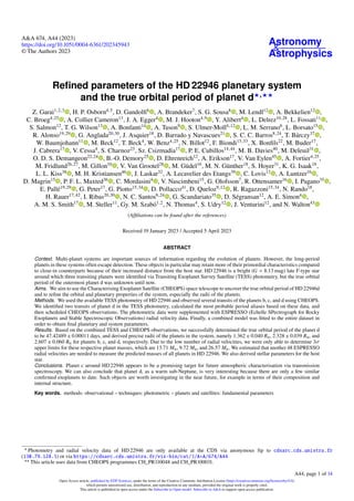
  • 7. Garai, Z., et al.: A&A proofs, manuscript no. aa45943-23 Table 6. Best-fitting and derived system and planetary parameters of the HD 22946 planetary system. Parameter (unit) Description HD 22946b HD 22946c HD 22946d Tc (BJDTDB) Reference mid-transit time 2 458 385.7321+0.0022 −0.0031 2 459 161.60861+0.00069 −0.00072 2 459 136.53720+0.00087 −0.00083 Porb (days) Orbital period 4.040295+0.000015 −0.000014 9.573083 ± 0.000014 47.42489+0.00010 −0.00011 b Impact parameter 0.21+0.11 −0.13 0.504+0.024 −0.026 0.456+0.026 −0.028 a/Rs Scaled semi-major axis 11.03 ± 0.12 19.61+0.22 −0.23 57.00 ± 0.66 a (au) Semi-major axis 0.05727+0.00085 −0.00082 0.1017+0.0015 −0.0014 0.2958+0.0044 −0.0042 Rp/Rs Planet-to-star radius ratio 0.01119+0.00031 −0.00032 0.01912+0.00026 −0.00027 0.02141+0.00046 −0.00045 tdur (days) Transit duration 0.1281+0.0026 −0.0037 0.1535+0.0015 −0.0014 0.2701+0.0019 −0.0020 Rp (R⊕) planet radius 1.362 ± 0.040 2.328+0.038 −0.039 2.607 ± 0.060 Mp (M⊕) planet mass(⋆) 13.71 9.72 26.57 Mp,est (M⊕) Estimated planet mass(♣) 2.42 ± 0.12 6.04 ± 0.17 7.32 ± 0.28 Mp,est (M⊕) Estimated planet mass(♡) 2.61 ± 0.27(†) 6.61 ± 0.17(‡) 7.90 ± 0.28(‡) ρp (g cm−3 ) planet density(⋆) 18.96 3.15 10.80 K (m s−1 ) RV semi-amplitude(⋆) 5.05 2.70 4.31 Ip (W m−2 ) Insolation flux 673 884+32 444 −31 606 213 337+10 270 −10 006 25 261+1216 −1184 Tsurf (K) Surface temperature(⋄) 1241 ± 14 931 ± 11 546 ± 6 TSM Transmission spectroscopy metric(♯) 43 ± 4 63 ± 2 43 ± 2 Notes. Based on the joint fit of the TESS and CHEOPS photometric data and RV observations. Table shows the best-fitting value of the given parameter and its ±1σ uncertainty. The fitted values correspond to quantile 0.50 (median) and the uncertainties to quantils ±0.341 in the parameter distributions obtained from the samples. (⋆) Only the 3σ upper limits are listed here due to the low number of the RV observations. (⋄) Assuming the albedo value of 0.2. (♣) Based on the relations presented by Chen & Kipping (2017), assuming that the planet radii are from the interval of 1.23 < Rp < 14.26 R⊕. (♡) Based on the relations presented by Otegi et al. (2020). (†) Assuming that ρp > 3.3 g cm−3 . (‡) Assuming that ρp < 3.3 g cm−3 . ♯ Based on the criteria set by Kempton et al. (2018), using the scale factor of 1.26, the stellar radius of Rs = 1.117 ± 0.009 R⊙ and J = 7.250 ± 0.027 mag (see Table 4). -0.1 -0.05 0 0.05 0.1 1200 1400 1600 1800 2000 2200 2400 2600 O-C [d] BJDTDB - 2457000 HD 22946b HD 22946c HD 22946d Fig. 1. Observed-minus-calculated (O-C) diagram of mid-transit times of the planets HD 22946b, HD 22946c, and HD 22946d obtained using the Allesfitter package. The O-C values are consistent with a linear ephemeris, which means no significant TTVs are present in the system. the obtained O–C diagram of the mid-transit times for planets b, c, and d from the Allesfitter package is depicted in Fig. 1. We can see that the O–C values are scattered around O–C = 0.0 d, which means that no significant TTVs are present in the system. 4. Final results and discussion The best-fitting and derived parameters from the combined model are listed in Table 6, and the model posteriors of the host star are summarised in Appendix A.2. The fitted TESS light curves from sector numbers 3, 4, 30, and 31 are depicted in the panels of Figs. 2 and 3. The CHEOPS individual observations overplotted with the best-fitting models are shown in the panels of Fig. 4. The RV observations fitted with a spectroscopic orbit are depicted in Fig. 5. Here, we present new ephemerides of the planetary orbits, which we calculated based on the combined model. Thanks to the combined TESS and CHEOPS observations, we were able to improve the reference mid-transit times and the orbital peri- ods of the planets compared to the discovery values. C22 derived the orbital period parameter values of Porb,b = 4.040301+0.000023 −0.000042 days and Porb,c = 9.573096+0.000026 −0.000023 days, and expected an orbital period of Porb = 46 ± 4 days for planet d, which was esti- mated based on the transit duration and depth along with stellar mass and radius through Kepler’s third law, assuming circular orbits. We confirmed this prediction, finding an orbital period for planet d of Porb = 47.42489 ± 0.00011 days. The improved ratios of the orbital periods are Porb,c/Porb,b = 2.37 and Porb,d/Porb,c = 4.95. Based on the Kepler database, the adjacent planet pairs in multiple systems show a broad overall peak between period ratios of 1.5 and 2, followed by a declining tail to larger period ratios. In addition, there appears to be a sizeable peak just inte- rior to the period ratio 5 (Steffen & Hwang 2015); therefore, we can say that the period ratios in HD 22946 fall into statistics and the seemingly large orbital gap between planets c and d is not anomalous. In the combined model, we determined the impact parame- ter b, which is the projected relative distance of the planet from the stellar disk centre during the transit midpoint in units of Rs. Converting these parameter values to the orbit inclination angle values we can obtain i = 88.90+0.16 −0.05 deg, i = 88.52+0.08 −0.07 deg, and i = 89.54+0.02 −0.03 deg for planets b, c, and d, respectively. For comparison, we note that the corresponding discovery values are ib = 88.3+1.1 −1.2 deg and ic = 88.57+0.86 −0.53 deg. The inclination A44, page 7 of 14
  • 8. A&A 674, A44 (2023) 0.999 0.9992 0.9994 0.9996 0.9998 1 1.0002 1.0004 1.0006 1.0008 1.001 1385 1390 1395 1400 1405 Relative flux BJDTDB - 2457000 TESS observations - Sector No. 03 Averaged data Full model 0.999 0.9992 0.9994 0.9996 0.9998 1 1.0002 1.0004 1.0006 1.0008 1.001 1385 1390 1395 1400 1405 Relative flux BJDTDB - 2457000 TESS observations - Sector No. 03 Averaged data Transit model 0.999 0.9992 0.9994 0.9996 0.9998 1 1.0002 1.0004 1.0006 1.0008 1.001 1410 1415 1420 1425 1430 1435 Relative flux BJDTDB - 2457000 TESS observations - Sector No. 04 Averaged data Full model 0.999 0.9992 0.9994 0.9996 0.9998 1 1.0002 1.0004 1.0006 1.0008 1.001 1410 1415 1420 1425 1430 1435 Relative flux BJDTDB - 2457000 TESS observations - Sector No. 04 Averaged data Transit model 0.999 0.9992 0.9994 0.9996 0.9998 1 1.0002 1.0004 1.0006 1.0008 1.001 2115 2120 2125 2130 2135 2140 Relative flux BJDTDB - 2457000 TESS observations - Sector No. 30 Averaged data Full model 0.999 0.9992 0.9994 0.9996 0.9998 1 1.0002 1.0004 1.0006 1.0008 1.001 2115 2120 2125 2130 2135 2140 Relative flux BJDTDB - 2457000 TESS observations - Sector No. 30 Averaged data Transit model Fig. 2. TESS observations of the transiting planets HD 22946b, HD 22946c, and HD 22946d from sector numbers 3, 4, and 30 overplotted with the best-fitting model. This model was derived based on the entire CHEOPS and TESS photometric dataset and the RV observations from ESPRESSO via joint analysis of the data. The left-hand panels show the non-detrended data overplotted with the full model, while the right-hand panels show the detrended data overplotted with the transit model. We averaged the TESS data for better visualisation of the transit events using a running average with steps and width of 0.009 and 0.09 day, respectively. We note that an interruption in communications between the instrument and spacecraft occurred at 2 458 418.54 BJDTDB, resulting in an instrument turn-off until 2 458 421.21 BJDTDB. No data were collected during this period. angle of planet d was not determined by C22. According to the improved parameter values, it seems that only the orbits of planets b and c are well aligned. planet d is probably not in the same plane as planets b and c. Based on the combined TESS and CHEOPS photometry observations, we redetermined the radii of the planets, which are 1.362 ± 0.040 R⊕, 2.328 ± 0.039 R⊕, and 2.607 ± 0.060 R⊕ for planets b, c, and d, respectively. The CHEOPS observa- tions are an added value, because compared to the corresponding parameter values presented in C22 (Rp,b = 1.72 ± 0.10 R⊕, Rp,c = 2.74 ± 0.14 R⊕, and Rp,d = 3.23 ± 0.19 R⊕), there is a notice- able improvement in radius precision. Using TESS and CHEOPS photometry observations, the uncertainties on the planet radius parameter values were decreased by ∼50%, 68%, and 61% for A44, page 8 of 14
  • 9. Garai, Z., et al.: A&A proofs, manuscript no. aa45943-23 0.999 0.9992 0.9994 0.9996 0.9998 1 1.0002 1.0004 1.0006 1.0008 1.001 2145 2150 2155 2160 2165 2170 Relative flux BJDTDB - 2457000 TESS observations - Sector No. 31 Averaged data Full model 0.999 0.9992 0.9994 0.9996 0.9998 1 1.0002 1.0004 1.0006 1.0008 1.001 2145 2150 2155 2160 2165 2170 Relative flux BJDTDB - 2457000 TESS observations - Sector No. 31 Averaged data Transit model Fig. 3. As in Fig. 2, but for the TESS sector number 31. planets b, c, and d, respectively. We also note that the parameter values from this work are in stark contrast to those derived by C22; these authors found significantly larger radii, that is, larger by ∼21%, 15%, and 19% for planets b, c, and d, respectively. We believe this may be due to a misunderstanding of the LimbDarkLightCurve function in exoplanet. The function requires the planetary radius Rp in solar radii rather than the planet-to-star radius ratio Rp/Rs. When misused, the result is an inflation of Rp/Rs and Rp values by a factor of Rs/R⊕, which in this case is a factor of about 15%–21%. This mistake can be seen most clearly in C22, when comparing the models shown in Fig. 5 with the implied depths in Table 4 (likely derived from the radius ratio), which are inflated by this factor. Such a mis- take was also evident during the reanalysis of the BD+40 2790 (TOI-2076) system (Osborn et al. 2022). According to the radius valley at ∼1.5–2.0 R⊕, which separates super-Earths and sub-Neptunes (Fulton et al. 2017; Van Eylen et al. 2018; Martinez et al. 2019; Ho & Van Eylen 2023), and based on the refined planet radii, we find that planet b is a super-Earth, and planets c and d are similar in size and are sub-Neptunes, in agreement with C22. It is well known that small exoplanets have bimodal radius distri- bution separated by the radius valley. Potential explanations focus on atmospheric-escape-driven mechanisms, such as photo- evaporation; see for example Owen (2019). The models showed that those planets that have radius below 1.5 R⊕ were plan- ets that initially had hydrogen/helium atmospheres, but ulti- mately lost them due to atmospheric escape, while those just above 2.0 R⊕ had hydrogen/helium atmosphere masses of ∼1% of the core mass. Having HD 22946 planets on either side of the valley means that planet b could be a photo-evaporated version of planets c and d. Recently, Luque & Pallé (2022) presented a brand new approach, arguing that the density of planets might provide more information than planet radii alone and proposing that a density gap separates rocky from water- rich planets. For M dwarf systems, these authors found that rocky planets form within the ice line while water worlds formed beyond the ice line and migrated inwards. Given that theoretical models predict similar results for stars of other types, this sce- nario could also be possible in the case of the planets orbiting HD 22946. Due to the low number of RVs, here we present only the 3σ upper limits for the planet masses in agreement with the discoverers. C22 obtained the 3σ upper mass limits of about 11 M⊕, 14.5 M⊕, and 24.5 M⊕ for planets b, c, and d, respectively, from the same spectroscopic observations. The 3σ upper limits for the planet masses from this work are Mp,b = 13.71 M⊕, Mp,c = 9.72 M⊕, and Mp,d = 26.57 M⊕. Similarly to the discoverers, we obtained very different upper mass lim- its for planets c and d, although they have similar planet radii, which could be due to a somewhat different internal structure of these planets. Applying the relations of Chen & Kipping (2017) and Otegi et al. (2020), we also re-estimated the planet masses, which were previously forecasted by the discoverers as 6.29 ± 1.30 M⊕, 7.96 ± 0.69 M⊕, and 10.53 ± 1.05 M⊕ for planets b, c, and d, respectively. The improved parameter values are pre- sented in Table 6. Furthermore, taking into account the estimated planet masses calculated based on the relations of Otegi et al. (2020), we predicted the number of additional RV measure- ments required to achieve a 3σ detection on each mass using the Radial Velocity Follow-up Calculator12 (RVFC; see Cloutier et al. 2018), and the RV simulator (Wilson et al., in prep.). Based on these simulations, we obtained that another 27, 24, and 48 ESPRESSO RVs are needed to measure the pre- dicted masses of planets b, c, and d, respectively. The expected RV semi-amplitudes assuming the estimated planet masses are Kb = 1.10 ± 0.12 m s−1 , Kc = 2.08 ± 0.10 m s−1 , and Kd = 1.46 ± 0.08 m s−1 . C22 also probed the planets from the viewpoint of future atmospheric characterisation using the transmission spec- troscopy metric (TSM); see Eq. (1) in Kempton et al. (2018). The authors obtained the TSM values of 65 ± 10, 89 ± 16, and 67 ± 14 for planets b, c, and d, respectively. We revised these values based on the results from the present work. The improved TSM values (see Table 6) do not satisfy the recommended value of TSM > 90 for planets with a radius of 1.5 < Rp < 10 R⊕. On the other hand, given that this threshold is set very rigorously, in agreement with the discoverers, we can note that planet c could be a feasible target for transmission spectroscopy observations with future atmospheric characterisation missions, such as the planned Ariel space observatory (Tinetti et al. 2021). Finally, we discuss the relevance of planet d among the known population of similar exoplanets. HD 22946d represents a warm sub-Neptune. Based on the NASA Exoplanet Archive13 (Akeson et al. 2013), there are 5272 confirmed exoplanets up to 22 February 2023, but only 63 planets out of 5272 are 12 See http://maestria.astro.umontreal.ca/rvfc/ 13 See https://exoplanetarchive.ipac.caltech.edu/index. html A44, page 9 of 14
  • 10. A&A 674, A44 (2023) 0.9992 0.9996 1 1.0004 1.0008 2504.6 2504.7 2504.8 2504.9 2505 2505.1 Relative flux 1st CHEOPS visit - HD 22946b Full model 0.9988 0.9992 0.9996 1 1.0004 1.0008 2505.8 2505.9 2506 2506.1 2506.2 2506.3 Relative flux BJDTDB - 2457000 2nd CHEOPS visit - HD 22946c Full model 0.9992 0.9996 1 1.0004 1.0008 2504.6 2504.7 2504.8 2504.9 2505 2505.1 Relative flux 1st CHEOPS visit - HD 22946b Transit model 0.9988 0.9992 0.9996 1 1.0004 1.0008 2505.8 2505.9 2506 2506.1 2506.2 2506.3 Relative flux BJDTDB - 2457000 2nd CHEOPS visit - HD 22946c Transit model 0.9992 0.9996 1 1.0004 1.0008 2512.8 2512.9 2513 2513.1 2513.2 2513.3 Relative flux 3rd CHEOPS visit - HD 22946b Full model 0.9992 0.9996 1 1.0004 1.0008 2516.9 2517 2517.1 2517.2 2517.3 Relative flux BJDTDB - 2457000 5th CHEOPS visit - HD 22946b Full model 0.9992 0.9996 1 1.0004 1.0008 2512.8 2512.9 2513 2513.1 2513.2 2513.3 Relative flux 3rd CHEOPS visit - HD 22946b Transit model 0.9992 0.9996 1 1.0004 1.0008 2516.9 2517 2517.1 2517.2 2517.3 Relative flux BJDTDB - 2457000 5th CHEOPS visit - HD 22946b Transit model 0.9984 0.9988 0.9992 0.9996 1 1.0004 1.0008 2515.6 2515.7 2515.8 2515.9 2516 2516.1 Relative flux BJDTDB - 2457000 4th CHEOPS visit - HD 22946c,d Full model - planet c Full model - planet d Full model 0.9984 0.9988 0.9992 0.9996 1 1.0004 1.0008 2515.6 2515.7 2515.8 2515.9 2516 2516.1 Relative flux BJDTDB - 2457000 4th CHEOPS visit - HD 22946c,d Transit model - planet c Transit model - planet d Full transit model Fig. 4. Individual CHEOPS observations of the transiting planets HD 22946b, HD 22946c, and HD 22946d. The observed light curves are overplot- ted with the best-fitting model. This model was derived based on the entire CHEOPS and TESS photometric dataset and the RV observations from ESPRESSO via joint analysis of the data. The left-hand panels show the non-detrended data overplotted with the full model, while the right-hand panels show the detrended data overplotted with the transit model. In the case of the fourth CHEOPS visit, as the multiple transit feature, the individual transit models of planets c and d are also shown in addition to the summed model. sub-Neptune sized (1.75 < Rp < 3.5 R⊕) and transiting bright stars (G ≤ 10 mag). Only 7 planets out of 63 have orbital peri- ods longer than 30 days and only 4 planets out of 7 have an equilibrium temperature of below 550 K. Three planets have a lower insolation flux than planet d, namely TOI-2076d (Osborn et al. 2022), HD 28109d (Dransfield et al. 2022), and HD 191939 (Badenas-Agusti et al. 2020). HD 22946d is there- fore an interesting target for future follow-up observations. One of the questions to be answered in the near future is the compo- sition and internal structure of sub-Neptune-type planets. Using CHEOPS observations, we determined the radius of planet d with high accuracy. Its true mass could be determined with another 48 ESPRESSO RV measurements according to the esti- mate we present above. A combination of mass and radius gives the overall density, which will be an important step forward towards understanding sub-Neptunes. A44, page 10 of 14
  • 11. Garai, Z., et al.: A&A proofs, manuscript no. aa45943-23 -8 -6 -4 -2 0 2 4 6 8 10 1510 1520 1530 1540 1550 1560 1570 RV [m/s] BJDTDB - 2457000 +/-1σ +/-2σ Obs. with +/-3σ RV model Fig. 5. RV observations taken at ESPRESSO fitted with a spectroscopic orbit (red line). The 1σ and 2σ uncertainties of the model are plotted as coloured areas. The uncertainties of the individual RV data points correspond to a 3σ interval. 5. Conclusions Based on the combined TESS and CHEOPS observations, we refined several parameters of the HD 22946 planetary system. First of all, we improved the ephemerides of the planetary orbits in comparison with the discovery values. We can confirm that planets b and c have short orbital periods below 10 days, namely 4.040295 ± 0.000015 days and 9.573083 ± 0.000014 days, respectively. The third planet, HD 22946d, has an orbital period of 47.42489 ± 0.00011 days, which we were able to derive based on additional CHEOPS observations. Furthermore, based on the combined TESS and CHEOPS observations, we derived precise radii for the planets, which are 1.362 ± 0.040 R⊕, 2.328 ± 0.039 R⊕, and 2.607 ± 0.060 R⊕ for planets b, c, and d, respectively. On the one hand, we can confirm the conclusion of the discoverers that the planetary system consists of a super- Earth, and planets c and d are sub-Neptunes. On the other hand, we find the planet radii values to be in tension with the values presented in the discovery paper, which is very probably due to misuse of the software by the discoverers. The low number of ESPRESSO RV measurements allowed us to derive only the 3σ upper limits for the planet masses, which are 13.71 M⊕, 9.72 M⊕, and 26.57 M⊕ for planets b, c, and d, respectively. We also investigated the planets from the viewpoint of possible future follow-up observations. First of all, we can con- clude that more RV observations are needed to improve the planet masses in this system. The applied spectroscopic observa- tions allowed us to derive precise stellar parameters of the host star and to fit an initial spectroscopic orbit to the RV data, but there is ample room for improvement in this way. We estimated that another 48 ESPRESSO RVs are needed to measure the pre- dicted masses of all planets in HD 22946. planet c could be a suitable target for future atmospheric characterisation via trans- mission spectroscopy. We can also conclude that planet d as a warm sub-Neptune is very interesting, because there are only a few similar confirmed exoplanets to date. Thanks to the syn- ergy of TESS and CHEOPS missions, there is a growing sample of planets, such as HD 22946d. Such objects are worth inves- tigating in the near future, for example in order to investigate their composition and internal structure. Finally, we can mention that future photometric and/or spectroscopic observations could also be oriented to searching for further possible planets in this system. Acknowledgements. We thank the anonymous reviewer for the helpful comments and suggestions. CHEOPS is an ESA mission in partnership with Switzerland with important contributions to the payload and the ground segment from Austria, Belgium, France, Germany, Hungary, Italy, Portugal, Spain, Sweden, and the United Kingdom. The CHEOPS Consortium would like to gratefully acknowledge the support received by all the agencies, offices, universities, and industries involved. Their flexibility and willingness to explore new approaches were essential to the success of this mission. This paper includes data collected with the TESS mission, obtained from the MAST data archive at the Space Telescope Science Institute (STScI). Funding for the TESS mission is provided by the NASA Explorer Program. STScI is operated by the Association of Universities for Research in Astronomy, Inc., under NASA contract NAS 5-26555. This research has made use of the Exoplanet Follow-up Observation Program (ExoFOP; DOI: 10.26134/ExoFOP5) website, which is operated by the California Institute of Technology, under contract with the National Aeronautics and Space Administration under the Exoplanet Explo- ration Program. This work has made use of data from the European Space Agency (ESA) mission Gaia (https://www.cosmos.esa.int/gaia), processed by the Gaia Data Processing and Analysis Consortium (DPAC, https://www.cosmos.esa.int/web/gaia/dpac/consortium). Funding for the DPAC has been provided by national institutions, in particular the insti- tutions participating in the Gaia Multilateral Agreement. Z.G. acknowledges the support of the Hungarian National Research, Development and Innovation Office (NKFIH) grant K-125015, the PRODEX Experiment Agreement No. 4000137122 between the ELTE Eötvös Loránd University and the European Space Agency (ESA-D/SCI-LE-2021-0025), the VEGA grant of the Slovak Academy of Sciences No. 2/0031/22, the Slovak Research and Development Agency contract No. APVV-20-0148, and the support of the city of Szombathely. Gy.M.Sz. acknowledges the support of the Hungarian National Research, Development and Innovation Office (NKFIH) grant K-125015, a PRODEX Institute Agreement between the ELTE Eötvös Loránd University and the European Space Agency (ESA-D/SCI-LE-2021-0025), the Lendület LP2018- 7/2021 grant of the Hungarian Academy of Science and the support of the city of Szombathely. A.Br. was supported by the SNSA. A.C.C. acknowledges support from STFC consolidated grant numbers ST/R000824/1 and ST/V000861/1, and UKSA grant number ST/R003203/1. B.-O.D. acknowledges support from the Swiss State Secretariat for Education, Research and Innovation (SERI) under contract number MB22.00046. This project has received funding from the European Research Council (ERC) under the European Union’s Horizon 2020 research and innovation programme (project FOUR ACES; grant agreement No 724427). It has also been carried out in the frame of the National Centre for Competence in Research PlanetS supported by the Swiss National Science Foundation (SNSF). D.E. acknowledges financial support from the Swiss National Science Foundation for project 200021_200726. D.G. gratefully acknowledges financial support from the CRT foundation under Grant No. 2018.2323 “Gaseousor rocky? Unveiling the nature of small worlds”. This work was also partially supported by a grant from the Simons Foundation (PI Queloz, grant number 327127). This work has been carried out within the framework of the NCCR PlanetS supported by the Swiss National Science Foundation under grants 51NF40_182901 and 51NF40_205606. I.R.I. acknowledges support from the Spanish Ministry of Science and Innovation and the European Regional Development Fund through grant PGC2018-098153-B-C33, as well as the support of the Generalitat de Catalunya/CERCA programme. This work was granted access to the HPC resources of MesoPSL financed by the Région Île-de-France and the project Equip@Meso (reference ANR-10-EQPX-29-01) of the programme Investissements d’Avenir supervised by the Agence Nationale pour la Recherche. K.G.I. and M.N.G. are the ESA CHEOPS Project Scientists and are responsible for the ESA CHEOPS Guest Observers Programme. They do not participate in, or contribute to, the definition of the Guaranteed Time Programme of the CHEOPS mission through which observations described in this paper have been taken, nor to any aspect of target selection for the programme. The Belgian participation to CHEOPS has been supported by the Belgian Federal Science Policy Office (BELSPO) in the framework of the PRODEX Program, and by the University of Liège through an ARC grant for Concerted Research Actions financed by the Wallonia-Brussels Federation; L.D. is an F.R.S.-FNRS Postdoctoral Researcher. L.M.S. gratefully acknowledges financial support from the CRT foundation under Grant No. 2018.2323 “Gaseous or rocky? Unveiling the nature of small worlds”. This project was supported by the CNES. M.F. and C.M.P. gratefully acknowledge the support of the Swedish National Space Agency (DNR 65/19, 174/18). M.G. is an F.R.S.-FNRS Senior Research Associate. M.L. acknowledges support of the Swiss National Science Foundation under grant number PCEFP2_194576. N.A.W. acknowledges UKSA grant ST/R004838/1. This work was supported by FCT – Fundação para a Ciência e a Tecnologia through national funds and by FEDER through COMPETE2020 – Programa Operacional Competitividade e Internacionalizacão by these grants: UID/FIS/04434/2019, UIDB/04434/2020, UIDP/04434/2020, PTDC/FIS-AST/32113/2017 & POCI-01-0145-FEDER- 032113, PTDC/FIS-AST/28953/2017 & POCI-01-0145-FEDER-028953, A44, page 11 of 14
  • 12. A&A 674, A44 (2023) PTDC/FIS-AST/28987/2017 & POCI-01-0145-FEDER-028987, O.D.S.D. is supported in the form of work contract (DL 57/2016/CP1364/CT0004) funded by national funds through FCT. P.M. acknowledges support from STFC research grant number ST/M001040/1. We acknowledge support from the Spanish Ministry of Science and Innovation and the European Regional Development Fund through grants ESP2016-80435-C2-1-R, ESP2016-80435-C2-2-R, PGC2018-098153-B-C33, PGC2018-098153-B-C31, ESP2017-87676-C5-1-R, MDM-2017-0737 Unidad de Excelencia Maria de Maeztu-Centro de Astrobiología (INTA-CSIC), as well as the support of the Generalitat de Catalunya/CERCA programme. The MOC activities have been supported by the ESA contract No. 4000124370. S.H. gratefully acknowledges CNES funding through the grant 837319. S.C.C.B. acknowledges support from FCT through FCT contracts nr. IF/01312/2014/CP1215/CT0004. S.G.S. acknowl- edges support from FCT through FCT contract no. CEECIND/00826/2018 and POPH/FSE (EC). A.C.C. and T.W. acknowledge support from STFC consolidated grant numbers ST/R000824/1 and ST/V000861/1, and UKSA grant number ST/R003203/1. V.V.G. is an F.R.S-FNRS Research Associate. X.B., S.C., D.G., M.F. and J.L. acknowledge their role as ESA-appointed CHEOPS science team members. Y.A. and M.J.H. acknowledge the support of the Swiss National Fund under grant 200020_172746. L.Bo., V.Na., I.Pa., G.Pi., R.Ra. and G.Sc. acknowledge support from CHEOPS ASI-INAF agreement n. 2019-29-HH.0. NCS acknowledges support from the European Research Council through the grant agreement 101052347 (FIERCE). This work was supported by FCT – Fundação para a Ciência e a Tecnologia through national funds and by FEDER through COMPETE2020 – Programa Operacional Competitividade e Internacionalização by these grants: UIDB/04434/2020; UIDP/04434/2020. A.T. thanks the Science and Technology Facilities Council (STFC) for a PhD studentship. P.E.C. is funded by the Austrian Science Fund (FWF) Erwin Schroedinger Fellowship, program J4595-N. References Akeson, R. L., Chen, X., Ciardi, D., et al. 2013, PASP, 125, 989 Allard, F. 2014, IAU Symp., 299, 271 Badenas-Agusti, M., Günther, M. N., Daylan, T., et al. 2020, AJ, 160, 113 Benz, W., Broeg, C., Fortier, A., et al. 2021, Exp. Astron., 51, 109 Bonfanti, A., Ortolani, S., Piotto, G., & Nascimbeni, V. 2015, A&A, 575, A18 Bonfanti, A., Ortolani, S., & Nascimbeni, V. 2016, A&A, 585, A5 Bonfanti, A., Delrez, L., Hooton, M. J., et al. 2021, A&A, 646, A157 Cacciapuoti, L., Inno, L., Covone, G., et al. 2022, A&A, 668, A85 Castelli, F., & Kurucz, R. L. 2003, IAU Symp., 210, A20 Chen, J., & Kipping, D. 2017, ApJ, 834, 17 Claret, A. 2018, A&A, 618, A20 Claret, A. 2021, RNAAS, 5, 13 Cloutier, R., Doyon, R., Bouchy, F., & Hébrard, G. 2018, AJ, 156, 82 Cooke, B. F., Pollacco, D., & Bayliss, D. 2019, A&A, 631, A83 Cooke, B. F., Pollacco, D., Anderson, D. R., et al. 2021, MNRAS, 500, 5088 Cutri, R. M., Skrutskie, M. F., van Dyk, S., et al. 2003, VizieR Online Data Catalog: II/246 Delrez, L., Ehrenreich, D., Alibert, Y., et al. 2021, Nat. Astron., 5, 775 Dobos, V., Charnoz, S., Pál, A., Roque-Bernard, A., & Szabó, G. M. 2021, PASP, 133, 094401 Dransfield, G., Triaud, A. H. M. J., Guillot, T., et al. 2022, MNRAS, 515, 1328 Foreman-Mackey, D., Agol, E., Ambikasaran, S., & Angus, R. 2017, AJ, 154, 220 Foreman-Mackey, D., Luger, R., Agol, E., et al. 2021, J. Open Source Softw., 6, 3285 Fulton, B. J., Petigura, E. A., Howard, A. W., et al. 2017, AJ, 154, 109 Gaia Collaboration (Brown, A. G. A., et al.) 2021, A&A, 649, A1 Gaia Collaboration (Vallenari, A., et al.) 2023, A&A, in press, https://doi. org/10.1051/0004-6361/202243940 Guerrero, N. M., Seager, S., Huang, C. X., et al. 2021, ApJS, 254, 39 Günther, M. N., & Daylan, T. 2019, Astrophysics Source Code Library [record ascl:1903.003] Günther, M. N., & Daylan, T. 2021, ApJS, 254, 13 Ho, C. S. K., & Van Eylen, V. 2023, MNRAS, 519, 4056 Hord, B. J., Colón, K. D., Berger, T. A., et al. 2022, AJ, 164, 13 Hoyer, S., Guterman, P., Demangeon, O., et al. 2020, A&A, 635, A24 Kempton, E. M. R., Bean, J. L., Louie, D. R., et al. 2018, PASP, 130, 114401 Kipping, D. 2018, RNAAS, 2, 223 Kipping, D. M., Spiegel, D. S., & Sasselov, D. D. 2013, MNRAS, 434, 1883 Kurucz, R. L. 1993a, SYNTHE spectrum synthesis programs and line data, CD- ROM No. 18 (Cambridge, MA: Smithsonian Astrophysical Observatory) Kurucz, R. L. 1993b, SYNTHE spectrum synthesis programs and line data (Astrophysics Source Code Library) Lacedelli, G., Malavolta, L., Borsato, L., et al. 2021, MNRAS, 501, 4148 Lacedelli, G., Wilson, T. G., Malavolta, L., et al. 2022, MNRAS, 511, 4551 Lindegren, L., Bastian, U., Biermann, M., et al. 2021, A&A, 649, A4 Lissauer, J. J., Marcy, G. W., Rowe, J. F., et al. 2012, ApJ, 750, 112 Luque, R., & Pallé, E. 2022, Science, 377, 1211 Marigo, P., Girardi, L., Bressan, A., et al. 2017, ApJ, 835, 77 Martinez, C. F., Cunha, K., Ghezzi, L., & Smith, V. V. 2019, ApJ, 875, 29 Maxted, P. F. L., Ehrenreich, D., Wilson, T. G., et al. 2022, MNRAS, 514, 77 Mayor, M., & Queloz, D. 1995, Nature, 378, 355 Nesvorný, D., & Morbidelli, A. 2008, ApJ, 688, 636 Osborn, H. P., Bonfanti, A., Gandolfi, D., et al. 2022, A&A, 664, A156 Osborn, H. P., Nowak, G., Hébrard, G., et al. 2023, MNRAS, 523, 3069 Otegi, J. F., Bouchy, F., & Helled, R. 2020, A&A, 634, A43 Owen, J. E. 2019, Annu. Rev. Earth Planet. Sci., 47, 67 Pepe, F., Molaro, P., Cristiani, S., et al. 2014, Astron. Nachr., 335, 8 Ricker, G. R. 2014, JAAVSO, 42, 234 Salmon, S. J. A. J., Van Grootel, V., Buldgen, G., Dupret, M. A., & Eggenberger, P. 2021, A&A, 646, A7 Salvatier, J., Wieckiâ, T. V., & Fonnesbeck, C. 2016, Astrophysics Source Code Library [record ascl:1610.016] Santos, N. C., Sousa, S. G., Mortier, A., et al. 2013, A&A, 556, A150 Scuflaire, R., Théado, S., Montalbán, J., et al. 2008, Ap&SS, 316, 83 Skrutskie, M. F., Cutri, R. M., Stiening, R., et al. 2006, AJ, 131, 1163 Sneden, C. A. 1973, Ph.D. Thesis, The University of Texas at Austin, USA Sousa, S. G. 2014, in Determination of Atmospheric Parameters of B-, A-, Fand G-Type Stars, eds. E. Niemczura, B. Smalley, & W. Pych (Berlin: Springer), 297 Sousa, S. G., Santos, N. C., Israelian, G., Mayor, M., & Monteiro, M. J. P. F. G. 2007, A&A, 469, 783 Sousa, S. G., Santos, N. C., Adibekyan, V., Delgado-Mena, E., & Israelian, G. 2015, A&A, 577, A67 Sousa, S. G., Adibekyan, V., Delgado-Mena, E., et al. 2021, A&A, 656, A53 Stassun, K. G., Oelkers, R. J., Pepper, J., et al. 2018, AJ, 156, 102 Stefánsson, G., Kopparapu, R., Lin, A., et al. 2020, AJ, 160, 259 Steffen, J. H., & Hwang, J. A. 2015, MNRAS, 448, 1956 Szabó, G. M., Gandolfi, D., Brandeker, A., et al. 2021, A&A, 654, A159 Szabó, G. M., Garai, Z., Brandeker, A., et al. 2022, A&A, 659, A7 Tinetti, G., Eccleston, P., Haswell, C., et al. 2021, ArXiv e-prints [arXiv:2104.04824] Tuson, A., Queloz, D., Osborn, H. P., et al. 2023, MNRAS, 523, 3090 Ulmer-Moll, S., Osborn, H. P., Tuson, A., et al. 2023, A&A, 674, A43 Van Eylen, V., & Albrecht, S. 2015, ApJ, 808, 126 Van Eylen, V., Agentoft, C., Lundkvist, M. S., et al. 2018, MNRAS, 479, 4786 Van Eylen, V., Albrecht, S., Huang, X., et al. 2019, AJ, 157, 61 Weiss, L. M., Marcy, G. W., Petigura, E. A., et al. 2018, AJ, 155, 48 Wilson, T. G., Goffo, E., Alibert, Y., et al. 2022, MNRAS, 511, 1043 Wright, E. L., Eisenhardt, P. R. M., Mainzer, A. K., et al. 2010, AJ, 140, 1868 1 MTA-ELTE Exoplanet Research Group, 9700 Szombathely, Szent Imre h. u. 112, Hungary e-mail: zgarai@ta3.sk 2 ELTE Gothard Astrophysical Observatory, 9700 Szombathely, Szent Imre h. u. 112, Hungary 3 Astronomical Institute, Slovak Academy of Sciences, 05960 Tatranská Lomnica, Slovakia 4 Physikalisches Institut, University of Bern, Gesellsschaftstrasse 6, 3012 Bern, Switzerland 5 Department of Physics and Kavli Institute for Astrophysics and Space Research, Massachusetts Institute of Technology, Cambridge, MA 02139, USA 6 Dipartimento di Fisica, Universita degli Studi di Torino, via Pietro Giuria 1, 10125, Torino, Italy 7 Department of Astronomy, Stockholm University, AlbaNova Uni- versity Center, 10691 Stockholm, Sweden 8 Instituto de Astrofisica e Ciencias do Espaco, Universidade do Porto, CAUP, Rua das Estrelas, 4150-762 Porto, Portugal 9 Astrophysics Group, Cavendish Laboratory, University of Cambridge, J.J. Thomson Avenue, Cambridge CB3 0HE, UK 10 Astrobiology Research Unit, Université de Liège, Allée du Six-Août 19C, 4000 Liège, Belgium 11 Space Research Institute, Austrian Academy of Sciences, Schmiedlstrasse 6, 8042 Graz, Austria A44, page 12 of 14
  • 13. Garai, Z., et al.: A&A proofs, manuscript no. aa45943-23 12 Observatoire Astronomique de l’Université de Genève, Chemin Pegasi 51, Versoix, Switzerland 13 Centre for Exoplanet Science, SUPA School of Physics and Astron- omy, University of St Andrews, North Haugh, St Andrews KY16 9SS, UK 14 Space Research Institute, Austrian Academy of Sciences, Schmiedlstrasse 6, 8042 Graz, Austria 15 INAF, Osservatorio Astronomico di Padova, Vicolo dell’Osservatorio 5, 35122 Padova, Italy 16 Department of Astrophysics, University of Vienna, Tuerkenschanzs- trasse 17, 1180 Vienna, Austria 17 Institute of Planetary Research, German Aerospace Center (DLR), Rutherfordstrasse 2, 12489 Berlin, Germany 18 European Space Agency (ESA), European Space Research and Technology Centre (ESTEC), Keplerlaan 1, 2201 AZ Noordwijk, The Netherlands 19 Instituto de Astrofisica de Canarias, 38200 La Laguna, Tenerife, Spain 20 Institut d’Estudis Espacials de Catalunya (IEEC), 08034 Barcelona, Spain 21 Depto. de Astrofisica, Centro de Astrobiologia (CSIC-INTA), ESAC campus, 28692 Villanueva de la Cañada (Madrid), Spain 22 Université Grenoble Alpes, CNRS, IPAG, 38000 Grenoble, France 23 Université de Paris, Institut de physique du globe de Paris, CNRS, 75005 Paris, France 24 Departamento de Fisica e Astronomia, Faculdade de Ciencias, Uni- versidade do Porto, Rua do Campo Alegre, 4169-007 Porto, Portugal 25 Center for Space and Habitability, University of Bern, Gesellschaftsstrasse 6, 3012 Bern, Switzerland 26 Leiden Observatory, University of Leiden, PO Box 9513, 2300 RA Leiden, The Netherlands 27 Department of Space, Earth and Environment, Chalmers University of Technology, Onsala Space Observatory, 43992 Onsala, Sweden 28 Space sciences, Technologies and Astrophysics Research (STAR) Institute, Université de Liège, 19C Allée du Six-Août, 4000 Liège, Belgium 29 Departamento de Astrofisica, Universidad de La Laguna, 38206 La Laguna, Tenerife, Spain 30 Institut de Ciencies de l’Espai (ICE, CSIC), Campus UAB, Can Magrans s/n, 08193 Bellaterra, Spain 31 Aix–Marseille Univ., CNRS, CNES, LAM, 38 rue Frédéric Joliot-Curie, 13388 Marseille, France 32 IMCCE, UMR8028 CNRS, Observatoire de Paris, PSL Univ., Sorbonne Univ., 77 av. Denfert-Rochereau, 75014 Paris, France 33 Max Planck Institute for Extraterrestrial Physics, Giessenbachstrasse 1, 85748 Garching bei München, Germany 34 Dipartimento di Fisica e Astronomia “Galileo Galilei”, Universita degli Studi di Padova, Vicolo dell’Osservatorio 3, 35122 Padova, Italy 35 INAF, Osservatorio Astrofisico di Catania, Via S. Sofia 78, 95123 Catania, Italy 36 Astrophysics Group, Keele University, Staffordshire ST5 5BG, UK 37 Admatis, 5. Kandó Kálmán Street, 3534 Miskolc, Hungary 38 Konkoly Observatory, Research Centre for Astronomy and Earth Sciences, 1121 Budapest, Konkoly Thege Miklós út 15–17, Hungary 39 Institut d’astrophysique de Paris, UMR7095 CNRS, Université Pierre-et-Marie-Curie, 98bis blvd. Arago, 75014 Paris, France 40 Centre for Mathematical Sciences, Lund University, Box 118, 22100 Lund, Sweden 41 Department of Physics, University of Warwick, Gibbet Hill Road, Coventry CV4 7AL, UK 42 Center for Astronomy and Astrophysics, Technical University Berlin, Hardenberstrasse 36, 10623 Berlin, Germany 43 Institute of Astronomy, University of Cambridge, Madingley Road, Cambridge CB3 0HA, UK 44 INAF, Osservatorio Astrofisico di Torino, Via Osservatorio 20, 10025 Pino Torinese, TO, Italy 45 Department of Space and Climate Physics, Mullard Space Science Laboratory, Holmbury St Mary RH5 6NT, UK 46 Brorfelde Observatory, Observator Gyldenkernes Vej 7, 4340 Tøl- løse, Denmark A44, page 13 of 14
  • 14. A&A 674, A44 (2023) Appendix A: Additional tables Table A.1. Best-fitting GP hyperparameters and detrending parameters. Parameter [unit] Description Value+1σ −1σ log σCHEOPS [ppt] log of scatter in the CHEOPS data −2.384+0.057 −0.061 log σTESS [ppt] log of scatter in the TESS data −2.845+0.024 −0.023 φω0,CHEOPS [1/deg] typical frequency of variation in the shared CHEOPS roll-angle GP 1.70+0.19 −0.16 ω0,TESS [1/d] frequency for the TESS SHOTerm GP kernel 1.87+0.10 −0.09 φS0,CHEOPS scaled power in the shared CHEOPS roll-angle GP 0.0062+0.0010 −0.0009 S 0,TESS scaled power in the TESS SHOTerm GP kernel 0.0066+0.0010 −0.0008 φpower,CHEOPS power in the shared CHEOPS roll-angle GP 0.052+0.020 −0.013 φlengthscale,CHEOPS [deg] typical lengthscale of variation in the shared CHEOPS rollangle GP 3.68+0.38 −0.37 d f/d(time)1st,CHEOPS linear detrending parameter for time trend vs. flux – 1st CHEOPS visit 0.075 ± 0.011 d f/d(bg)1st,CHEOPS linear detrending parameter for background vs. flux – 1st CHEOPS visit −0.026 ± 0.036 d2 f/d(bg)2 1st,CHEOPS quadratic detrending parameter for background vs. flux – 1st CHEOPS visit 0.0278 ± 0.0025 d f/d(centroid x)1st,CHEOPS linear detrending parameter for x centroid vs. flux – 1st CHEOPS visit 0.0386+0.0080 −0.0078 d f/d(centroid y)1st,CHEOPS linear detrending parameter for y centroid vs. flux – 1st CHEOPS visit −0.0458+0.0083 −0.0084 d f/d(centroid x)2nd,CHEOPS linear detrending parameter for x centroid vs. flux – 2nd CHEOPS visit 0.202+0.044 −0.045 d2 f/d(centroid x)2 2nd,CHEOPS quadratic detrending parameter for x centroid vs. flux – 2nd CHEOPS visit −0.0304 ± 0.0083 d f/d(time)3rd,CHEOPS linear detrending parameter for time trend vs. flux – 3rd CHEOPS visit 0.015 ± 0.010 d f/d(centroid y)3rd,CHEOPS linear detrending parameter for y centroid vs. flux – 3rd CHEOPS visit −0.0357+0.0074 −0.0075 d f/d(time)4th,CHEOPS linear detrending parameter for time trend vs. flux – 4th CHEOPS visit 0.103 ± 0.013 d f/d(centroid y)4th,CHEOPS linear detrending parameter for y centroid vs. flux – 4th CHEOPS visit −0.061 ± 0.010 d2 f/d(centroid y)2 4th,CHEOPS quadratic detrending parameter for y centroid vs. flux – 4th CHEOPS visit 0.0086 ± 0.0019 xmean,1st,CHEOPS [ppt] the average offset of the median-normalised flux – 1st CHEOPS visit 0.007 ± 0.011 xmean,2nd,CHEOPS [ppt] the average offset of the median-normalised flux – 2nd CHEOPS visit 0.066 ± 0.011 xmean,3rd,CHEOPS [ppt] the average offset of the median-normalised flux – 3rd CHEOPS visit 0.039 ± 0.010 xmean,4th,CHEOPS [ppt] the average offset of the median-normalised flux – 4th CHEOPS visit 0.314 ± 0.014 xmean,5th,CHEOPS [ppt] the average offset of the median-normalised flux – 5th CHEOPS visit 0.061 ± 0.011 xmean,TESS [ppt] the average offset of the median-normalised flux in TESS data 0.0179+0.0085 −0.0084 Notes. Based on the joint fit of the TESS and CHEOPS photometric data, and RV observations. The table shows the best-fitting value of the given parameter and its ±1σ uncertainty. The fitted values correspond to quantile 0.50 (median) and the uncertainties to quantils ±0.341 in the parameter distributions obtained from the samples. Table A.2. As in Table A.1, but for model posteriors of the host HD 22946. Parameter [unit] Description Value+1σ −1σ Teff [K] effective temperature 6167+64 −63 log g [cgs] log of surface gravity 4.358 ± 0.016 u1,TESS quadratic LD coefficient 0.196 ± 0.077 u2,TESS quadratic LD coefficient 0.244 ± 0.086 u1,CHEOPS quadratic LD coefficient 0.346+0.081 −0.079 u2,CHEOPS quadratic LD coefficient 0.291+0.089 −0.090 Rs [R⊙] stellar radius 1.1161+0.0088 −0.0089 Ms [M⊙] stellar mass 1.105 ± 0.038 γ [m s−1 ] system RV 16 854.48+0.82 −0.76 A44, page 14 of 14