Linear Programming Module - A Conceptual Framework.

1. Linear Programming Module- A Conceptual Framework
Prepared
By
P.K. Viswanathan
Introduction:
An economist faces the problem of making an optimum allocation of resources among
competing projects. A business-planning manager has to decide how many units of each
product be produced to maximize profit subject to constraints on production capacity and
demand for these products. We need a model that can help us to find the best solution in
the context of constraints that are operating on the problem. Linear programming
provides solutions to such problems. The word programming implies planning.
Learning Objectives:
After reading this module, you will be able to:
 Know what is Linear Programming (LP)

 Formulate Linear Programming Problems

 Use Graphical Method to Solve LP

 Appreciate Shadow Prices and Interpret

 Appreciate Computer Solutions for Large LP problems

Contents:
1. What is Linear Programming?
2. Steps in formulating LP Problems
3. Solution-Graphical Method
4. Computer Solution
5. A Comprehensive Case on LP
6. Module Summary
7. Review Questions
1. What is Linear Programming?
Linear Programming (LP) is concerned with the best way of allocating scarce resources
among competing ends. The word optimization is used in the context of either
maximizing or minimizing an objective function. Organizations do have problems such
as minimizing cost of production, or maximizing the profit. The resources that are
available in limited quantities are called constraints and the optimization will have to take
place subject to the constraints the organization has.
1

2. "Programming" here means planning and has nothing to do with computer programming.
The word 'linear" is very important. Linear implies that the objective function and
constraints are all linear namely the variables are raised to the power 1 only. The
constraints could be of three types: 1) less than or equal to 2) equal to and 3) greater than
or equal to. Symbolically, they are represented as respectively.
, ,
To put it succinctly, linear programming is a very widely used OR model that maximizes
or minimizes an objective function subject to a number of limiting factors called
constraints. All relationships among the variables are linear. That is objective function,
and constraints are all linear. Another requirement of LP is that all variables must be non-
negative (0 or positive). You cannot have a negative solution in linear programming
although mathematically you may get negative solutions for the decision variables.
Some Examples where LP is applied

An advertising company wants to maximize exposure of a client’s product and
has a choice of advertising in different media that include TV, Radio, and
magazines. These media charge different advertising costs. The ad company has
to achieve its objective of maximizing exposure subject to the constraints of ad
budget, minimum and maximum number of ads in the various media. LP can help
the company solve this problem.
 furniture manufacturer producing a number of items would like to maximize his
A
profit. He has certain commitments to his customers in the form of minimum and
maximum quantities to be supplied for each item. Also in his plant, the available
production time in each of the 3 departments is limited. LP can help him find an
optimum product mix that can maximize his total profit.

Applications of linear programming are plenty. Product mix problem, media
planning, transportation problem, blending problem, scheduling of nurses and
doctors to the patients in a hospital, and capital investment are among the many
where linear programming can be applied.
2. Steps in formulating LP Problems

Identify the decision variables.
Decision variables are those for which you are trying to find the solution.
Identifying the decision variables is important in solving an LP problem

Formulate the objective function in terms of the decision variables
If the organization’s goal is to maximize profit, the objective function will be a
maximization case. Likewise, in a blending problem, if the aim is to minimize
cost, then the objective function will be a minimization case. At any rate, you
must be able to express the objective function in terms of the decision variables.
2

3. 
Formulate the constraints in terms of the decision variables.
Constraints represent limitations on resources. They will also have to be written in
terms of the decision variables.
Note: As the solution for the decision variables should not turn out to be negative, you
have to specify that they are zero or positive. This is termed as non-negativity constraint.
In any LP problem, it is generally understood that all the decision variables are non-
negative.
Example: One of the divisions of a small-scale unit manufactures two products. Both the
products require two raw materials and the consumption per unit production is given
below:
Table -Consumption in kg per unit production
Product 1 Product 2 Maximum
Availability
of Raw
Materials
(kg)
Raw Material1 2 3 18
Raw Material2 1 1 8
Further, it is known from market research that product 1 cannot be sold more than 4 units.
The profit per unit of product 1 is $ 15, and product 2 is $ 21. You will have to help this
small-scale unit decide how many units of product 1 and product 2 to produce so as to
maximize the total profit.
Formulation
Identify the decision variables:
Let x1 be the number of units of product 1 to be produced
Let x2 be the number of units of product 2 to be produced
Formulate the objective function in terms of the decision variables:
The profit per unit of product is $. 15 and product 2 is $.21. If you produce x1 units of
product 1 and x2 units of product 2, then the total profit =15x1 + 21x2 . This has to be
maximized. In linear programming terminology, we write the objective function as
Z = 15x1 + 21x2 . Z is to be maximized.
Formulate the constraints in terms of the decision variables:
The maximum quantity of product 1 that can be sold is 4 units. So
x1  (Sales constraint)
4
3

4. The maximum availability of raw material 1 is 18 kg. To produce x1 units of product1 and
x2 units of product 2, you need 2x1 + 3x2 kg. So,
2x1 + 3x2 18 (raw material 1 availability) (see table of consumption above)
Similarly we can work out the raw material availability constraint for raw material 2. And
it is
x1 + x2 8 (raw material 2 availability)
Complete formulation for the example:
Maximize Z = 15x1 + 21x2
Subject to:
x1 4
2x1 + 3x2 18
x1 + x2 8
And x1, x2 0(non-negativity)
Inline Question: Linear programming is one of the computer programming languages.
True or False.
Answer: The statement is false. The word programming means planning and linear means
the relationships among the variables are raised to the power 1. This has nothing to do with
computer programming language.
Assumptions in Linear Programming:
1) Proportionality: Because we assume linear relationship among variables in LP,
proportionality is inevitable. Suppose you need 5 kg of input to produce one unit.
Then to produce two units, you need 10 kg of input. This is not necessarily true.
2) Additivity: When we formulate the constraints, we add resource requirements of
the decision variables. We ignore the interaction term in the expression. Interaction
measures the effect of any combination of decision variables.
3) Divisibility: Divisibility does not guarantee integer solutions. In a particular
problem, fractional solution does not make sense. For example, in a product mix
problem, you may get a solution that says produce 10.3 units of model 1 and 14.4
4

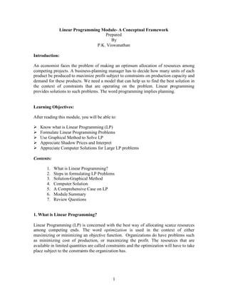
5. units of model 2. It does not make sense. Rounding to the whole number
sometimes may vitiate the solutions. Of course you have a technique called integer
linear programming that can help you solve problems where you are looking for
integer solutions.
4) Certainty: In linear programming, you assume all variables are known without any
doubt. Thus, you assume a deterministic or certainty scenario. But in reality, you
may have to assess carefully the magnitude of uncertainty.
3. Solution-Graphical Method
Graphical method of solving a linear programming model is possible only for two
variables. To get a feel for linear programming, graphical method is extremely useful.
Let us take the same example used for formulating LP model.
Example Problem:Graphical Solution
Constraint Lines and Feasibility Region
Drawn in a combined manner
x2
8
x1 + x2= 8
7
6 A(0,6) X 1=4
5
4
B (4, 3 1/3)
3 Feasibility Region
2
2 x1 + 3x2 =18
1
D(0,0) C(4,0)
x1
1 2 3 4 5 6 7
7 8
8 9
9 10
10
5

6. Please see the feasibility region in the diagram bounded by thick lines with corner points
co-ordinates marked by A(0,6), B(4, 3 1/3), C(4,0) and D(0,0). This is the region that
satisfies all the three constraints. Co-ordinates for B is obtained by solving the two
equations X1 = 4 and 2X1+3X 2 =18. Do not read the co-ordinates from the graph. You may
not get the accuracy. The word feasibility is important here. It says that every pair of co-
ordinate points in this region is a feasible solution to the problem given. But, what is the
optimum solution? See next.
Optimal Solution
In any linear programming problem the optimum
solution when it exists is always one of the corner
points in the feasibility region. Select that corner
point which gives the maximum Z value. (Note: For
minimization case select that corner point that gives
the minimum Z value). In our case we need to select
the maximum Z value.
Corner Point Z Value : Z= 15x1 + 21x2
A(0,6) 126
B(4, 3 1/3) Optimum 130
C(4,0) 60
D(0,0) 0
6

7. The optimum solution that maximizes the profit is to produce 4 units of product 1 and
3 1/3 units of product 2. The maximum profit is $. 130.
Inline question: If the example problem discussed is a minimization problem, what is the
optimum solution?
Answer: Take that corner point that gives the minimum value of Z. Omit the trivial
solution D(0,0) that says don’t produce any thing. Z is minimum for C(4,0). The value of Z
=60. The optimum solution is to produce 4 units of product 1 and 0 units of product 2.
Assignment: Solve the following LP problem graphically:
Maximize Z = 8X1 + 10X2
Subject to: 8X1 + 4X2 240
6X1 +12X2 360
X1, X2 0
4. Computer Solution:
Graphical method just provides some insights into linear programming. It can solve
problems having two variables only. In practice, complex problems involving more than
two variables are encountered. The efficient way of solving such problems is to use
“Solver” in Microsoft Excel. You can get output giving insights into shadow prices and
sensitivity analysis apart from the usual optimum solution. The method used for solving
linear programming problems is called “simplex method” discovered by Dantiz. Doing this
manually in practice is not only time consuming but also error prone. Computer solution is
simple and best.
The emphasis in this module is on your ability to formulate a linear programming model
for a given problem and then solve it using “Solver”. The technical terms associated with
linear programming purely from a mathematical perspective will be avoided. For a
manager, a problem well formulated is half solved. The simple slogan I would popularize is
“Excel in formulating any LP problem and solve it using Excel”.
Before we move on to solving some complex LP problems, let us first solve a simple
problem using solver. Take the example used for graphical method. Follow the step-by-step
procedure. The formulation of this problem on the spreadsheet is given below:
7

8. Model Formulation on the spreadsheet
Explanation on the Formulation:
This is a crucial step in using solver. Column A is used for labeling the linear programming
vocabulary. Decision Variables appear in cell A2. In Column B and C, Product1 and
Product 2 are labeled. Corresponding to Row 2 and columns B and C values 1 and 1 are
entered. These are the initial values of the decision variables X1 and X 2 we have used while
formulating the LP model. These initial values are varied by solver to get the optimum
values of X1 and X2. Please remember, solver cannot accept X1 and X2 in the respective
cells. Please note that you are at liberty to use your own labeling and Excel is flexible in
this regard.
In A4 cell Objective Function is written. Against this label, under Column B and C values
15 and 21 are entered. These are the unit profits of the two products. F3 is labeled as Total
Profit and F4 gives the profit that is obtained by multiplying the coefficients of the
objective function with the initial values of the decision variables. That is (15)(1)+21(1)
=36. In order that Excel understands this, you create a formula in F4(target cell)
=B4*B2+C4*C2. Excel will vary the values of B2 and C2 to get the optimum values of
Product1 and Product2.
8

9. Then we label in Column A in Row 6 Constraints. Under this we further label the
individual constraints namely Sales for Product1, Raw material1 availability, and Raw
material2 availability. In Column B and C we enter the coefficients of the decision
variables corresponding to these constraints. The value 1 is entered under column B
corresponding to Sales for Product1 and value 0 is entered under column C for Product2. In
Column D corresponding to Sales for product1, the value 1 appears. This is calculated by
the formula =B7*B2+C7*C2 and this is 1. In Column E corresponding to Sales for
Product1, we label the symbol < = meaning less than or equal to constraint. This labeling is
done for our own understanding and Excel ignores this. In Column F corresponding to
Sales for Product1, we have entered the value 4. Now if you look at the entire Row 4, for
the constraint Sales for Product1, you are saying B7*B2+C7*C2 < = 4. This is same as
saying X1 < =4. Likewise the constraints on raw material 1 and raw material 2 are worked
out. For better clarity, spreadsheet showing model equations are given next:
Spreadsheet Giving Model Equations
9

10. Solution: Now you are ready to invoke solver. Click Tools, and click Solver. You get
In “Set Target Cell” highlight F4 that contains the objective function. In “Equal To” click
Max because you want to maximize the objective function. “By Changing Cells” is
Solver’s way of saying that the initial values of the decision variables are varied until
optimal solution is reached. You highlight the cells B2:C2. You now get
Solution continues:
10

11. You now come to “Subject to the Constraints”. Solver accepts all the three types of
constraints (< =, =, > =). When you develop a model, you better arrange the constraints
according to types in the spreadsheet itself. That is all < = are done first; then > = and then
=. This will save a lot of time. You can enter a set of constraints together in Solver by
highlighting the appropriate cells. Here all the constraints are < = and are arranged in that
order. You click “Add” and you get
In “Cell Reference” you highlight D7:D9. Click < =. Then highlight cells F7:F9 for
constraint values. You have now entered all constraints. You get now
Click OK and you get
Complete Formulation of LP Model for the Example
11

12. The last two things that remain to be done by you is to tell Solver that you are solving a
linear programming model and the decision variables are non-negative. Click Options.
Then click Assume Linear Model and Assume Non-Negative. After this, you click Solve
and you get
Now click OK. You get the solution shown next.
Model Giving Optimal Solution
As you can see the optimum solution is to produce 4 units of Product1 and 3.33 units of
Product2. The maximum total profit is $. 130. Constraints 1 and 2 are fully exhausted
meaning that the resources are fully utilized. In the LP parlance, the word slack is used.
Here slack is 0. Slack represents the unused quantity of a resource. For constraint3, there is
12

13. a slack of 0.67 kg that was unutilized. This cannot be helped as things stand. Any attempt
we make to use more of this will not give a profit better than $.130.
Sensitivity Analysis
Finding the solution to a linear programming model is only a first step. A manager would
like to know how sensitive the solution is to changes in inputs and assumptions. Let us
interpret the sensitivity analysis output given by solver for the LP problem just solved.
When you click solve, you actually get
If you now press OK, you get the optimum solution. Before clicking OK, highlight
Sensitivity and then click OK. You get
13

14. Shadow Price:

The shadow price gives the incremental increase in profit when the right hand side
value of a constraint is increased by one unit, and the decrease in profit when the
right hand side value of a constraint is decreased by one unit. Shadow prices play a
key role in evaluating the worth of increasing the resources and also new product
evaluation. Let us interpret the shadow prices for our example.

Shadow price corresponding to constraint 1 namely Sales for Product1 is seen to be
=1. This means that the objective function (total profit) will increase or decrease by
$1 if the sale quantity for product1 is increased or decreased by $1. From a
marketing angle every additional unit sold on product 1 will increase the profit by
$1.

Shadow price corresponding to constraint 2 is 7. This means that an increase or
decrease of 1 kg in availability of raw material 2 will produce an increase or
decrease of $7 in the objective function. So, the moral of the story is that every
additional kg of raw material 2 made available will increase the profit by $7.

Shadow price for raw material 2 is 0. It does not make any impact on the objective
function.

Thus shadow prices for Sale of Product 1, Raw Material 1, and Raw Material 2 are
$1, $7, and $0 respectively.

The allowable increase and allowable decrease shown in the output indicates the
range for which the shadow prices will hold true.
Inline Question: For the example discussed, if the small-unit’s R&D department has
created a new product called Product 3. It is quite profitable, $25 per unit. It requires 4kg
of raw material 1 and 1 kg of raw material 2. Should Product 3 be produced?
Solution: The opportunity cost of producing one unit of Product 3 is:
(Shadow price of raw material 1)(Consumption of raw material 1 per unit production)
+(Shadow price of raw material 2)(Consumption of raw material 2 per unit production)
=$7 4+0 1=$28
This represents the opportunity cost that the company will have to forego by not producing
Product 1 and Product 2. The profit per unit of Product 3 is $25. Since this is less than
$28(opportunity cost of not producing Product 1 and Product 2), Product 3 should not be
produced.
14

15. 5. Comprehensive Case on LP
Programmers Recruitment Planning
A software company conducts a short applied certificate course in computer
programming for trainee programmers. Trained programmers are used as instructors in
the certificate course in the ratio of one for every ten trainee programmers recruited. The
certificate course lasts for one month. From past experience, it has been found that out of
ten trainee programmers hired, only six complete the certificate course successfully (the
unsuccessful trainee programmers are sent out).
Trained programmers are also needed for company's computer assignments and the
company's requirements for the next three months are as follows:
Month 1 200
Month 2 300
Month 3 350
In addition, the company requires 400 trained programmers in the beginning of Month 4.
There are 230 trained programmers available as of now.
Salary Details are:
Each Trainee Programmer Rs. 4000
Each Trained Programmer Rs. 7000
(Doing company’s computer
assignments or as instructor)
Each Trained Programmer
who remains idle Rs. 5000
(Union agreement prevents firing
Trained Programmers)
Decide and set up the hiring and training schedule of programmers, which will meet the
company's requirements at minimum cost
Problem Formulation for the Case:
•Identify the decision variables
Let X1 =Trained programmers functioning as instructors in Month 1
Let X2 =Trained programmers who remain idle in Month 1
Let X3= Trained programmers functioning as instructors in Month 2
Let X4= Trained programmers who remain idle in Month 2
Let X5= Trained programmers functioning as instructors in Month 3
Let X6 =Trained programmers who remain idle in Month 3
15

16. •Formulate the objective function
Minimize Z = 4000(10X1+10X3+10X5) +7000(X1+X3+X5)+5000(X2+X4+X6)
Z = Total Variable Cost. The salary to be paid to programmers in Month 1, Month 2, and
Month 3 are fixed cost that cannot be reduced. Hence, in the objective function, it is not
included. Simplifying Z = 47000X1+5000X2+47000X3+5000X4+47000X5+5000X6
Note: Because trained programmers are used as instructors in the course in the ratio of
one for every 10 trainee programmers recruited, the following are true:
10X1 trainee programmers are recruited in Month 1
10X3 trainee programmers are recruited in Month 2
10X5 trainee programmers are recruited in Month 3
•Formulate the constraints
230 = 200+X1+X2 (Month 1 constraint)
230+6X1 =300+X3+X4 (Month 2 constraint)
230+6X1+6X3 =350+X5+X6 (Month 3 constraint)
230+6X1+6X3+6X5 = 400 (Month 4 constraint)
Note: Out of 10X1 trainee programmers recruited, 6X1 are successful in the course in
Month 1 and are available for company’s computer assignments or functioning as
instructors in Month 2. Similarly those who are successful in completing the course in
Month 2, and Month 3 are available in the subsequent month for company’s computer
assignments or functioning as instructors
Upon simplification, the constraints are:
Month 1 X1+X2 = 30
Month 2 6X1-X3-X4 = 70
Month 3 6X1+6X3-X5-X6 = 120
Month 4 6X1+6X3+6X5 = 170
X1,X2,X3,X4,X5,X6 are 0 (Non-negativity)
Complete LP Formulation for the Example:
Minimize Z=47000X1+5000X2+47000X3+5000X4+47000X5+5000X6
Subject to constraints
X1+X2 = 30(Month 1)
6X1-X3-X4 = 70(Month 2)
6X1+6X3-X5-X6 = 120(Month 3)
6X1+6X3+6X5 = 170(Month 4)
X1, X2, X3, X4, X5, X6 are 0 (Non-negativity)
16

17. Inline Question: Obtain optimum solution for the case problem above using solver. You
show the initial model formulation on the spreadsheet and then the model solution.
Solution: Follow the step-by step procedure discussed in this module. It is just an
extension of the two-decision variables case to six-decision variables case. Every step
will be the same.
Spreadsheet Displaying Model Formulation
17

18. Spreadsheet Displaying Optimum Solution
As you can see that the minimum cost is Rs 1416531. The optimum values of the
decision variables are:
X1 =Trained programmers functioning as instructors in Month 1 = 13
X2 =Trained programmers who remain idle in Month 1 = 17
X3= Trained programmers functioning as instructors in Month 2 = 8
X4= Trained programmers who remain idle in Month 2 = 0
X5= Trained programmers functioning as instructors in Month 3 = 7
X6 =Trained programmers who remain idle in Month 3 = 0
We have rounded the values of the decision variables to integers as fractional values of
programmers are not possible. Please note that all constraints are fully satisfied when you
take the fractional values.
18

19. 6. Module Summary
This module has introduced you to a very useful resource optimization tool called linear
programming. Specifically this module focused on:

Meaning, definition, and examples of linear programming

Steps in formulating linear programming model

Explaining the LP model formulation steps through an example

Problem formulation is key to solution

Computer solution using Solver of Microsoft Excel

Explaining computer solution through an example

Sensitivity analysis as an important tool for mangers to see the changes in
solution as a result of changes in inputs and assumptions.

The role of shadow price in evaluating the worth of increasing or decreasing
resource quantities as well as the worth of a new product
 comprehensive case discussion on LP model formulation and computer solution
A
7. Review Questions (Test Items)
Discussion Topic
Analyze, criticize, and explain the following statement:
“ Linear programming is an oversimplification of real life problems. It assumes only one
objective function when organizations are facing multiple objectives”.
1) What is linear programming?
Answer: Linear programming is a technique in management science that
maximizes or minimizes an objective function subject to a number of limiting
factors called constraints.
2) What are the assumptions of a linear programming model?
19

20. Answer: The model assumes proportionality, additivity, divisibility, and
deterministic scenario.
3) What are the steps in a linear programming model formulation?
Answer: 1) Identify the decision variables 2) Formulate the objective function in
terms of the decision variables 3) Formulate the constraints in terms the decision
variables 4) Superimpose the non-negativity requirements on decision variables (0
or positive)
4) What is sensitivity analysis in LP?
Answer: Sensitivity analysis means how the linear programming model solution
reacts to changes in input parameters such as costs, prices, and resources. It
attempts to answer how sensitive the solution is to changes in inputs and
assumptions.
5) What is shadow price?
Answer: Shadow price gives the incremental increase in profit when the right
hand side value of a constraint is increased by one unit, and the decrease in profit
when the right hand side value of a constraint is decreased by one unit. Shadow
prices play a key role in evaluating the worth of increasing the resources and also
new product evaluation.
6) Mini Case:
Mr. Joseph, investment manager of Wizard Finance has $120000 to invest in new IT
stocks. Data on four chosen stocks are given below:
Stock Dividend Growth % Price per Share
1 1.5 30 35
2 0.75 25 45
3 2.0 28 40
4 0.5 35 55
Mr. Joseph has been asked to maximize growth in $ value excluding dividends of this
portfolio of shares in the coming year. It is Wizard’s policy to get at least $2500 as
annual dividend from this portfolio of shares. Wizard also wants to play safe by
stipulating the following conditions. Amount invested in stock 4 cannot be more than
55% of amount invested in stock 1. Further the company requires that at least 15% of
total investment be in stock 2.
Formulate and solve this case as a linear programming problem and obtain the
optimum solution-using Solver.
20

21. Solution:
Identify the decision variables
Let X1 = $ amount invested in Stock 1
Let X2 = $ amount invested in Stock 2
Let X3 = $ amount invested in Stock 3
Let X4 = $ amount invested in Stock 4
Formulate the objective function
From the wording of the problem, it is clear that Wizard would like to maximize the
growth of this portfolio of shares.
Maximize Z = 0.30X1+0.25X2+0.28X3+0.35X4
Formulate the constraints
Stock Dividend Growth % Price per Share
1 1.5 30 35
2 0.75 25 45
3 2.0 28 40
4 0.5 35 55
The amount set aside for investment is $120000. Hence the total amount invested
in the four shares has to be less than or equal to $120000.
X1+X2+X3+X4 < = 120000(Investment amount constraint)
The company specifies an annual dividend of at least $2500 for this portfolio of
shares. This is a bit tricky. Since we know dividends per share as well as the price
of each share. The annual dividend from this portfolio is =
 
1.5  0.75   
2.0  
0.5
   X1   
X2    X3   . This must be greater than or equal to
X4
 
35 45   
40  
55
$2500. Hence this constraint is
 
1.5  0.75   
2.0  
0.5
   X1   
X2    X3   > =2500(Dividend constraint). Upon
X4
 
35 45   40  
55
simplification this constraint becomes
0.43X1+0.017X2+0.050X3+0.009X4 > =2500(Dividend constraint)
21

22. Amount invested in Stock 4 cannot be more than 55% of amount invested in
Stock 1. This constraint can be written as
X4 < = 0.55X1. Simplifying this is written as
X4-0.55X1< =0(Safety constraint)
The last constraint is at least 15% of total amount invested must be in Stock2.
This can be written as
X2 > = 0.15(X1+X2+X3+X4). Simplifying this expression, this constraint becomes
–0.15X1+0.85X2-0.15X3-0.15X4 > = 0(Minimum amount in Stock 2 constraint)
Finally X1, X2, X3, X4 > = 0(Non-negativity)
Complete Model Structure (arranged according to the type of constraints)
Maximize Z = 0.30X1+0.25X2+0.28X3+0.35X4
Subject to
X1+X2+X3+X4 < = 120000(Investment amount constraint)
X4-0.55X1< =0(Safety constraint)
0.43X1+0.017X2+0.050X3+0.009X4 > =2500(Dividend constraint)
–0.15X1+0.85X2-0.15X3-0.15X4 > = 0(Minimum amount in Stock 2
constraint)
X1, X2, X3, X4 > = 0(Non-negativity)
Let us now get the solution from Excel using Solver.
22

23. Spreadsheet Displaying Model formulation
Optimum solution is given next.
23

24. Spreadsheet Displaying Optimum Solution
The optimum solution is to invest $65806 in Stock 1, $18000 in Stock 2, $0 in
Stock 3, and $36194 in Stock 4. The maximum growth = $36909. 68
Glossary:
Additivity: This is one of the assumptions of linear programming in which the
resources for the decision variables are added for getting the total resource.
Certainty: In linear programming, we assume all variables are known without
any doubt. That is, we assume a deterministic or certainty scenario.
Constraints: Restrictions in the form of resource limitations or requirement in a
linear programming problem.
Decision variables: Variables those are unknown for which solution is sought.
Divisibility: One of the assumptions of linear programming by which
the decision variables will have fractional solutions. This may not be meaningful
in situations where we need integer solutions.
24

25. Linear: This is one of the requirements of linear programming, which stipulates
that the objective function and constraints are all linear namely the variables are
raised to the power 1 only.
Linear Programming (LP): It is a very widely used OR model that maximizes
or minimizes an objective function subject to a number constraints. Linear
Programming is concerned with the best way of allocating scarce resources
among competing ends.
Nonnegativity Constraints: This is a requirement in linear programming that
says that the decision variables cannot have negative solutions. That is, they can
have only positive or zero values.
Objective Function: It is the goal of the organization written mathematically in
terms of the decision variables. This is either maximized or minimized.
Optimization: This word is used in the context of either maximizing or
minimizing an objective function.
Optimum Solution: The best values of the decision variables for a given linear
programming problem.
Programming: Programming in the context of LP means planning and has
nothing to do with computer programming.
Proportionality: This is another assumption in linear programming that says that
the value of the resources utilized are in direct proportion to the values of the
decision variables. This assumption is a sequel to the assumption of linearity of
objective function and constraints in LP.
Shadow Price: This gives the incremental increase in profit when the right hand
side value of a constraint is increased by one unit, and the decrease in profit when
the right hand side value of a constraint is decreased by one unit. Shadow prices
play a key role in evaluating the worth of increasing the resources and also new
product evaluation.
25