Shigley's Mechanical Engineering Design 9th Edition Solutions Manual

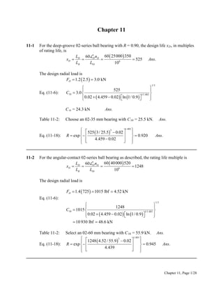
1. Chapter 11
11-1
For the deep-groove 02-series ball bearing with R = 0.90, the design life x D , in multiples
of rating life, is
L
60D nD 60  25000  350
xD  D 

 525 Ans.
LR
L10
106
The design radial load is
FD  1.2  2.5   3.0 kN
1/3
Eq. (11-6):


525


C10  3.0 
1/1.483 
 0.02   4.459  0.02  ln 1/ 0.9  





C 10 = 24.3 kN
Table 11-2:
Ans.
Choose an 02-35 mm bearing with C 10 = 25.5 kN.
Ans.
1.483
3


  525  3 / 25.5  0.02  
Eq. (11-18): R  exp  
Ans.
   0.920
4.459  0.02
 
 

 

______________________________________________________________________________
11-2
For the angular-contact 02-series ball bearing as described, the rating life multiple is
L
60D nD 60  40 000  520
xD  D 

 1248
LR
L10
106
The design radial load is
FD  1.4  725  1015 lbf  4.52 kN
Eq. (11-6):
1/3


1248


C10  1015 
1/1.483 
 0.02   4.459  0.02   ln 1/ 0.9  





 10 930 lbf  48.6 kN
Select an 02-60 mm bearing with C 10 = 55.9 kN. Ans.
1.483
3


 1248  4.52 / 55.9   0.02  
Eq. (11-18): R  exp  
Ans.
   0.945
4.439

 
 
 

______________________________________________________________________________
Table 11-2:
Chapter 11, Page 1/28

2. 11-3
For the straight-roller 03-series bearing selection, x D = 1248 rating lives from Prob. 11-2
solution.
FD  1.4  2235  3129 lbf  13.92 kN
 1248 
C10  13.92 

 1 
Table 11-3:
3/10
 118 kN
Select an 03-60 mm bearing with C 10 = 123 kN.
Ans.
1.483
10/3


 1248 13.92 /123  0.02  
Eq. (11-18): R  exp  
   0.917 Ans.
4.459  0.02
 
 
 
 
______________________________________________________________________________
11-4
The combined reliability of the two bearings selected in Probs. 11-2 and 11-3 is
R   0.945 0.917   0.867
Ans.
We can choose a reliability goal of 0.90  0.95 for each bearing. We make the
selections, find the existing reliabilities, multiply them together, and observe that the
reliability goal is exceeded due to the roundup of capacity upon table entry.
Another possibility is to use the reliability of one bearing, say R 1 . Then set the reliability
goal of the second as
R2 
0.90
R1
or vice versa. This gives three pairs of selections to compare in terms of cost, geometry
implications, etc.
______________________________________________________________________________
11-5
Establish a reliability goal of
contact ball bearing,
0.90  0.95 for each bearing. For an 02-series angular
1/3


1248


C10  1015 
1/1.483 
 0.02  4.439 ln 1/ 0.95 





 12822 lbf  57.1 kN
Select an 02-65 mm angular-contact bearing with C 10 = 63.7 kN.
1.483
3


 1248  4.52 / 63.7   0.02  
RA  exp  
   0.962
4.439
 
 
 
 
Chapter 11, Page 2/28

3. For an 03-series straight roller bearing,
3/10


1248


C10  13.92 
1/1.483 
 0.02  4.439  ln 1/ 0.95  





 136.5 kN
Select an 03-65 mm straight-roller bearing with C 10 = 138 kN.
 1248 13.92 /138 10/3  0.02 1.483 




RB  exp  
   0.953
4.439
 
 
 
 
The overall reliability is R = (0.962)(0.953) = 0.917, which exceeds the goal.
______________________________________________________________________________
11-6
For the straight cylindrical roller bearing specified with a service factor of 1, R = 0.95 and
F R = 20 kN.
60D nD 60  8000  950
L
xD  D 

 456
106
LR
L10
3/10


456


C10  20 
 145 kN
Ans.
1/1.483 
 0.02  4.439  ln 1/ 0.95  





______________________________________________________________________________
11-7
Both bearings need to be rated in terms of the same catalog rating system in order to
compare them. Using a rating life of one million revolutions, both bearings can be rated
in terms of a Basic Load Rating.
1/ a
Eq. (11-3):
L 
C A  FA  A 
 LR 
 8.96 kN
1/ a
  n 60 
 FA  A A 
 LR 
  3000  500  60  
 2.0 

106


1/3
Bearing B already is rated at one million revolutions, so C B = 7.0 kN. Since C A > C B ,
bearing A can carry the larger load.
Ans.
______________________________________________________________________________
11-8
F D = 2 kN, L D = 109 rev, R = 0.90
1/ a
1/3
 LD 
 109 
Eq. (11-3):
C10  FD 
  2  6   20 kN Ans.
 10 
 LR 
______________________________________________________________________________
Chapter 11, Page 3/28

4. 11-9
F D = 800 lbf,  D = 12 000 hours, n D = 350 rev/min, R = 0.90
 12 000  350  60  
  n 60 
Eq. (11-3):
C10  FD  D D   800 
  5050 lbf Ans
106
 LR 


______________________________________________________________________________
1/ a
1/3
11-10 F D = 4 kN,  D = 8 000 hours, n D = 500 rev/min, R = 0.90
 8 000  500  60  
  n 60 
Eq. (11-3):
C10  FD  D D   4 
  24.9 kN Ans
106
 LR 


______________________________________________________________________________
1/ a
1/3
11-11 F D = 650 lbf, n D = 400 rev/min, R = 0.95




 D = (5 years)(40 h/week)(52 week/year) = 10 400 hours
Assume an application factor of one. The multiple of rating life is
xD 
LD 10 400  400  60 

 249.6
LR
106
1/3


249.6


C10  1 650  
Eq. (11-6):
1/1.483 




 0.02  4.439 ln 1/ 0.95  

 4800 lbf Ans.
______________________________________________________________________________
11-12 F D = 9 kN, L D = 108 rev, R = 0.99
Assume an application factor of one. The multiple of rating life is
xD 
LD 108

 100
LR 106
1/3


100


C10  1 9  
Eq. (11-6):
1/1.483 
 0.02  4.439 ln 1/ 0.99  





 69.2 kN Ans.
______________________________________________________________________________
11-13 F D = 11 kips,  D = 20 000 hours, n D = 200 rev/min, R = 0.99
Assume an application factor of one. Use the Weibull parameters for Manufacturer 2 on
p. 608.
Chapter 11, Page 4/28

5. The multiple of rating life is
xD 
LD  20 000  200  60 

 240
LR
106
1/3


240


C10  111 
Eq. (11-6):
1/1.483 
 0.02  4.439 ln 1/ 0.99  





 113 kips Ans.
______________________________________________________________________________
11-14 From the solution to Prob. 3-68, the ground reaction force carried by the bearing at C is
R C = F D = 178 lbf. Use the Weibull parameters for Manufacturer 2 on p. 608.
xD 
LD 15000 1200  60 

 1080
LR
106
1/ a
Eq. (11-7):


xD
C10  a f FD 

1/ b
 x0    x0 1  RD  


1/3


1080
C10  1.2 178  

1/1.483
 0.02   4.459  0.02 1  0.95 



 2590 lbf Ans.
______________________________________________________________________________
11-15 From the solution to Prob. 3-69, the ground reaction force carried by the bearing at C is
R C = F D = 1.794 kN. Use the Weibull parameters for Manufacturer 2 on p. 608.
xD 
LD 15000 1200  60 

 1080
LR
106
1/ a
Eq. (11-7):


xD
C10  a f FD 

1/ b
 x0    x0 1  RD  


1/3


1080
C10  1.2 1.794  

1/1.483
 0.02   4.459  0.02 1  0.95 



 26.1 kN Ans.
______________________________________________________________________________
11-16 From the solution to Prob. 3-70, R Cz = –327.99 lbf, R Cy = –127.27 lbf
1/ 2
2
2
RC  FD   327.99    127.27    351.8 lbf


Use the Weibull parameters for Manufacturer 2 on p. 608.
Chapter 11, Page 5/28

6. xD 
LD 15000 1200  60 

 1080
LR
106
1/ a
Eq. (11-7):


xD
C10  a f FD 

1/ b
 xo    xo 1  RD  


1/3


1080
C10  1.2  351.8  

1/1.483
 0.02   4.459  0.02 1  0.95 



 5110 lbf Ans.
______________________________________________________________________________
11-17 From the solution to Prob. 3-71, R Cz = –150.7 N, R Cy = –86.10 N
1/2
2
2
RC  FD   150.7    86.10    173.6 N


Use the Weibull parameters for Manufacturer 2 on p. 608.
xD 
LD 15000 1200  60 

 1080
106
LR
1/ a
Eq. (11-7):


xD
C10  a f FD 

1/ b
 x0    x0 1  RD  


1/3


1080
C10  1.2 173.6  

1/1.483
 0.02   4.459  0.02 1  0.95 



 2520 N Ans.
______________________________________________________________________________
11-18 From the solution to Prob. 3-77, R Az = 444 N, R Ay = 2384 N

RA  FD  4442  23842

1/2
 2425 N  2.425 kN
Use the Weibull parameters for Manufacturer 2 on p. 608. The design speed is equal to
the speed of shaft AD,
d
125
nD  F ni 
191  95.5 rev/min
dC
250
xD 
LD 12 000  95.5  60 

 68.76
LR
106
1/ a
Eq. (11-7):


xD
C10  a f FD 

1/ b
 x0    x0 1  RD  


Chapter 11, Page 6/28

7. 1/3


68.76
C10  1 2.425  

1/1.483
 0.02   4.459  0.02 1  0.95 



 11.7 kN Ans.
______________________________________________________________________________
11-19 From the solution to Prob. 3-79, R Az = 54.0 lbf, R Ay = 140 lbf

RA  FD  54.02  1402

1/2
 150.1 lbf
Use the Weibull parameters for Manufacturer 2 on p. 608. The design speed is equal to
the speed of shaft AD,
d
10
nD  F ni   280   560 rev/min
dC
5
xD 
Eq. (11-7):
LD 14 000  560  60 

 470.4
LR
106


xD
C10  a f FD 

1/ b
 x0    x0 1  RD  


1/ a
3/10


470.4
C10  1150.1 

1/1.483
 0.02   4.459  0.02 1  0.98 



 1320 lbf Ans.
______________________________________________________________________________
11-20 (a) Fa  3 kN, Fr  7 kN, nD  500 rev/min, V  1.2
From Table 11-2, with a 65 mm bore, C 0 = 34.0 kN.
F a / C 0 = 3 / 34 = 0.088
From Table 11-1, 0.28  e  3.0.
Fa
3

 0.357
VFr 1.2  7 
Since this is greater than e, interpolating Table 11-1 with F a / C 0 = 0.088, we obtain
X 2 = 0.56 and Y 2 = 1.53.
Eq. (11-9):
Fe  X iVFr  Yi Fa   0.56 1.2  7   1.53 3  9.29 kN
F e > F r so use F e .
Ans.
(b) Use Eq. (11-7) to determine the necessary rated load the bearing should have to carry
the equivalent radial load for the desired life and reliability. Use the Weibull
parameters for Manufacturer 2 on p. 608.
Chapter 11, Page 7/28

8. xD 
LD 10 000  500  60 

 300
LR
106
1/ a


xD
Eq. (11-7): C10  a f FD 

1/ b
 x0    x0 1  RD  




300
C10  1 9.29  

1/1.483
 0.02   4.459  0.02 1  0.95 



 73.4 kN
1/3
From Table 11-2, the 65 mm bearing is rated for 55.9 kN, which is less than the
necessary rating to meet the specifications. This bearing should not be expected to meet
the load, life, and reliability goals.
Ans.
______________________________________________________________________________
11-21 (a) Fa  2 kN, Fr  5 kN, nD  400 rev/min, V  1
From Table 11-2, 30 mm bore, C 10 = 19.5 kN, C 0 = 10.0 kN
F a / C 0 = 2 / 10 = 0.2
From Table 11-1, 0.34  e  0.38.
Fa
2

 0.4
VFr 1 5 
Since this is greater than e, interpolating Table 11-1, with F a / C 0 = 0.2, we obtain X 2 =
0.56 and Y 2 = 1.27.
Ans.
Eq. (11-9): Fe  X iVFr  Yi Fa   0.56 1 5  1.27  2   5.34 kN
F e > F r so use F e .
(b) Solve Eq. (11-7) for x D .
 C
xD   10
 a f FD

a

1/ b
  x0    x0 1  RD  
 


3
 19.5 
 0.02   4.459  0.02 1  0.99 1/1.483 
xD  
 1 5.34   




xD  10.66
xD 
LD D nD  60 

LR
106
Chapter 11, Page 8/28

9. D 
   10.66 10   444 h
xD 106
6
Ans.
nD  60   400  60 
______________________________________________________________________________
11-22 Fr  8 kN, R  0.9, LD  109 rev
1/ a
Eq. (11-3):
L 
C10  FD  D 
 LR 
1/3
 109 
 8 6 
 10 
 80 kN
From Table 11-2, select the 85 mm bore. Ans.
______________________________________________________________________________
11-23 Fr  8 kN, Fa  2 kN, V  1, R  0.99
Use the Weibull parameters for Manufacturer 2 on p. 608.
xD 
LD 10 000  400  60 

 240
LR
106
First guess: Choose from middle of Table 11-1, X = 0.56, Y = 1.63
Eq. (11-9):
Fe  0.56 1 8   1.63  2   7.74 kN
F e < F r , so just use F r as the design load.
Eq. (11-7):


xD
C10  a f FD 

1/ b
 xo    xo 1  RD  


1/ a
1/3


240
C10  1 8  
  82.5 kN
1/1.483
 0.02   4.459  0.02 1  0.99 



From Table 11-2, try 85 mm bore with C 10 = 83.2 kN, C 0 = 53.0 kN
Iterate the previous process:
F a / C 0 = 2 / 53 = 0.038
0.22  e  0.24
Fa
2

 0.25  e
VFr 1 8 
Interpolate Table 11-1 with F a / C 0 = 0.038 to obtain X 2 = 0.56 and Y 2 = 1.89.
Table 11-1:
Eq. (11-9):
Fe  0.56(1)8  1.89(2)  8.26 > Fr
Eq. (11-7):


240
C10  1 8.26  

1/1.483
 0.02   4.459  0.02 1  0.99 



1/3
 85.2 kN
Chapter 11, Page 9/28

10. Table 11-2: Move up to the 90 mm bore with C 10 = 95.6 kN, C 0 = 62.0 kN.
Iterate again:
F a / C 0 = 2 / 62 = 0.032
Again, 0.22  e  0.24
Fa
2

 0.25  e
VFr 1 8 
Interpolate Table 11-1 with F a / C 0 = 0.032 to obtain X 2 = 0.56 and Y 2 = 1.95.
Table 11-1:
Eq. (11-9):
Fe  0.56(1)8  1.95(2)  8.38 > Fr
1/3


240
Eq. (11-7):
C10  1 8.38  
  86.4 kN
1/1.483
 0.02   4.459  0.02 1  0.99 



The 90 mm bore is acceptable. Ans.
______________________________________________________________________________
11-24 Fr  8 kN, Fa  3 kN, V  1.2, R  0.9, LD  108 rev
First guess: Choose from middle of Table 11-1, X = 0.56, Y = 1.63
Eq. (11-9):
Fe  0.56 1.2  8   1.63  3  10.3 kN
Fe  Fr
1/ a
Eq. (11-3):
L 
C10  Fe  D 
 LR 
1/3
 108 
 10.3  6 
 10 
 47.8 kN
From Table 11-2, try 60 mm with C 10 = 47.5 kN, C 0 = 28.0 kN
Iterate the previous process:
F a / C 0 = 3 / 28 = 0.107
0.28  e  0.30
Fa
3

 0.313  e
VFr 1.2  8 
Interpolate Table 11-1 with F a / C 0 = 0.107 to obtain X 2 = 0.56 and Y 2 = 1.46
Table 11-1:
Eq. (11-9):
Fe  0.56 1.2  8   1.46  3  9.76 kN > Fr
1/3
 108 
Eq. (11-3):
C10  9.76  6   45.3 kN
 10 
From Table 11-2, we have converged on the 60 mm bearing. Ans.
______________________________________________________________________________
Chapter 11, Page 10/28

11. 11-25 Fr  10 kN, Fa  5 kN, V  1, R  0.95
Use the Weibull parameters for Manufacturer 2 on p. 608.
xD 
LD 12 000  300  60 

 216
LR
106
First guess: Choose from middle of Table 11-1, X = 0.56, Y = 1.63
Eq. (11-9):
Fe  0.56 110   1.63  5   13.75 kN
F e > F r , so use F e as the design load.
Eq. (11-7):


xD
C10  a f FD 

1/ b
 x0    x0 1  RD  


1/ a
1/3


216
C10  113.75  

1/1.483
 0.02   4.459  0.02 1  0.95 



 97.4 kN
From Table 11-2, try 95 mm bore with C 10 = 108 kN, C 0 = 69.5 kN
Iterate the previous process:
F a / C 0 = 5 / 69.5 = 0.072
Table 11-1:
0.27  e  0.28
Fa
5

 0.5  e
VFr 110 
Interpolate Table 11-1 with F a / C 0 = 0.072 to obtain X 2 = 0.56 and Y 2 = 1.62  1.63
Since this is where we started, we will converge back to the same bearing. The 95 mm
bore meets the requirements. Ans.
______________________________________________________________________________
11-26 Note to the Instructor. In the first printing of the 9th edition, the design life was
incorrectly given to be 109 rev and will be corrected to 108 rev in subsequent printings.
We apologize for the inconvenience.
Fr  9 kN, Fa  3 kN, V  1.2, R  0.99
Use the Weibull parameters for Manufacturer 2 on p. 608.
xD 
LD 108

 100
LR 106
First guess: Choose from middle of Table 11-1, X = 0.56, Y = 1.63
Chapter 11, Page 11/28

12. Eq. (11-9):
Fe  0.56 1.2  9   1.63  3  10.9 kN
F e > F r , so use F e as the design load.
Eq. (11-7):


xD
C10  a f FD 

1/ b
 x0    x0 1  RD  


1/ a
1/3


100
C10  110.9  

1/1.483
 0.02   4.459  0.02 1  0.99 



 83.9 kN
From Table 11-2, try 90 mm bore with C 10 = 95.6 kN, C 0 = 62.0 kN. Try this bearing.
Iterate the previous process:
F a / C 0 = 3 / 62 = 0.048
0.24  e  0.26
Fa
3

 0.278  e
VFr 1.2  9 
Interpolate Table 11-1 with F a / C 0 = 0.048 to obtain X 2 = 0.56 and Y 2 = 1.79
Table 11-1:
Eq. (11-9):
Fe  0.56 1.2  9   1.79  3  11.4 kN  Fr
11.4
83.9  87.7 kN
10.9
From Table 11-2, this converges back to the same bearing. The 90 mm bore meets the
requirements. Ans.
______________________________________________________________________________
C10 
11-27 (a) nD  1200 rev/min, LD  15 kh, R  0.95, a f  1.2
From Prob. 3-72, R Cy = 183.1 lbf, R Cz = –861.5 lbf.
1/2
2
RC  FD  183.12   861.5    881 lbf


15000 1200  60 
L
xD  D 
 1080
LR
106
1/3


1080
Eq. (11-7): C10  1.2  881 

1/1.483
 0.02  4.439 1  0.95 



 12800 lbf  12.8 kips Ans.
(b) Results will vary depending on the specific bearing manufacturer selected. A general
engineering components search site such as www.globalspec.com might be useful as
a starting point.
______________________________________________________________________________
Chapter 11, Page 12/28

13. 11-28 (a) nD  1200 rev/min, LD  15 kh, R  0.95, a f  1.2
From Prob. 3-72, R Oy = –208.5 lbf, R Oz = 259.3 lbf.
1/ 2
2
RC  FD   259.32   208.5    333 lbf


15000 1200  60 
L
xD  D 
 1080
106
LR
1/3


1080
Eq. (11-7): C10  1.2  333 

1/1.483
 0.02  4.439 1  0.95 



 4837 lbf  4.84 kips Ans.
(b) Results will vary depending on the specific bearing manufacturer selected. A general
engineering components search site such as www.globalspec.com might be useful as
a starting point.
______________________________________________________________________________
11-29 (a) nD  900 rev/min, LD  12 kh, R  0.98, a f  1.2
From Prob. 3-73, R Cy = 8.319 kN, R Cz = –10.830 kN.
2 1/ 2
RC  FD  8.319 2   10.830    13.7 kN


12 000  900  60 
L
xD  D 
 648
LR
106
1/3


648
Eq. (11-7): C10  1.2 13.7  
  204 kN Ans.
1/1.483
 0.02  4.439 1  0.98 



(b) Results will vary depending on the specific bearing manufacturer selected. A general
engineering components search site such as www.globalspec.com might be useful as
a starting point.
______________________________________________________________________________
11-30 (a) nD  900 rev/min, LD  12 kh, R  0.98, a f  1.2
From Prob. 3-73, R Oy = 5083 N, R Oz = 494 N.

RC  FD  50832  4942
xD 

1/2
 5106 N  5.1 kN
LD 12 000  900  60 

 648
LR
106
1/3


648
Eq. (11-7): C10  1.2  5.1 
  76.1 kN Ans.
1/1.483
 0.02  4.439 1  0.98 



(b) Results will vary depending on the specific bearing manufacturer selected. A general
engineering components search site such as www.globalspec.com might be useful as
a starting point.
______________________________________________________________________________
Chapter 11, Page 13/28

14. 11-31 Assume concentrated forces as shown.
Pz  8  28   224 lbf
Py  8  35  280 lbf
T  224  2   448 lbf  in
T x  448  1.5 F cos 20  0
448
F
 318 lbf
1.5  0.940 
z
y
M O  5.75Py  11.5RA  14.25F sin 20  0
y
5.75  280   11.5RA  14.25  318 0.342   0
y
RA  5.24 lbf
y
z
M O  5.75 Pz  11.5 RA  14.25 F cos 20  0
z
5.75  224   11.5RA  14.25  318 0.940   0
1/2
2
2
RA   482    5.24  


z
z
z

F  RO  Pz  RA  F cos 20  0
z
RA  482 lbf;
 482 lbf
z
RO  224  482  318  0.940   0
z
RO  40.9 lbf
y
y
F y  RO  Py  RA  F sin 20  0
y
RO  280  5.24  318  0.342   0
y
RO  166 lbf
1/2
2
2
RO   40.9    166  


 171 lbf
So the reaction at A governs.
Reliability Goal: 0.92  0.96
FD  1.2  482   578 lbf
xD  35 000  350  60  / 106  735
1/3


735


C10  578 
1/1.483 
 0.02   4.459  0.02  ln 1/ 0.96  





 6431 lbf  28.6 kN
From Table 11-2, a 40 mm bore angular contact bearing is sufficient with a rating of
Chapter 11, Page 14/28

15. 31.9 kN.
Ans.
______________________________________________________________________________
11-32 For a combined reliability goal of 0.95, use 0.95  0.975 for the individual bearings.
xD 
40 000  420  60 
106
 1008
The resultant of the given forces are
R O = [(–387)2 + 4672]1/2 = 607 lbf
R B = [3162 + (–1615)2]1/2 = 1646 lbf
At O:
1/3


1008


C10  1.2  607  
Eq. (11-6):
1/1.483 
 0.02   4.459  0.02  ln 1/ 0.975  





 9978 lbf  44.4 kN
From Table 11-2, select an 02-55 mm angular-contact ball bearing with a basic load
rating of 46.2 kN. Ans.
At B:
3/10
Eq. (11-6):


1008


C10  1.2 1646  
1/1.483 
 0.02   4.459  0.02  ln 1/ 0.975  





 20827 lbf  92.7 kN
From Table 11-3, select an 02-75 mm or 03-55 mm cylindrical roller. Ans.
______________________________________________________________________________
11-33 The reliability of the individual bearings is R  0.98  0.9899
Chapter 11, Page 15/28

16. From statics,
T = (270  50) = (P 1  P 2 )125
= (P 1  0.15 P 1 )125
P 1 = 310.6 N,
P 2 = 0.15 (310.6) = 46.6 N
P 1 + P 2 = 357.2 N
FAy  357.2 sin 45  252.6 N  FAz
M
F
M
F
y
y
 850RE  300(252.6)  0  RE  89.2 N
z
O
y
y
y
 252.6  89.2  RO  0  RO  163.4 N
z
z
 850RE  700(320)  300(252.6)  0  RE  174.4 N
y
O
z
z
z
 174.4  320  252.6  RO  0  RO  107 N
RO 
 163.4 
2
RE 
 89.2 
  174.4   196 N
2
 107 2  195 N
2
The radial loads are nearly the same at O and E. We can use the same bearing at both
locations.
xD 
60 000 1500  60 
106
 5400
1/3
Eq. (11-6):


5400


C10  1 0.196  
1/1.483 
 0.02  4.439 ln 1/ 0.9899  





 5.7 kN
From Table 11-2, select an 02-12 mm deep-groove ball bearing with a basic load rating
of 6.89 kN. Ans.
______________________________________________________________________________
11-34
R  0.96  0.980
T  12(240 cos 20 )  2706 lbf  in
F
2706
 498 lbf
6 cos 25
In xy-plane:
z
y
M O  16(82.1)  30(210)  42 RC  0
Chapter 11, Page 16/28

17. y
RC  181 lbf
y
RO  82.1  210  181  111.1 lbf
In xz-plane:
y
z
M O  16(226)  30(451)  42 RC  0
z
RC  236 lbf
z
RO  226  451  236  11 lbf

 181
RO  111.12  112
RC
xD 
2
 236 2


1/ 2
 112 lbf
Ans.
1/ 2
 297 lbf
Ans.
50000  300  60 
106
 900
1/3
 C10 O


900


 1.2 112  
1/1.483 




 0.02  4.439 ln 1/ 0.980  

 1860 lbf  8.28 kN
1/3
 C10 C


900


 1.2  297  
1/1.483 




 0.02  4.439 ln 1/ 0.980  

 4932 lbf  21.9 kN
Bearing at O: Choose a deep-groove 02-17 mm. Ans.
Bearing at C: Choose a deep-groove 02-35 mm. Ans.
______________________________________________________________________________
11-35 Shafts subjected to thrust can be constrained by bearings, one of which supports the
thrust. The shaft floats within the endplay of the second (roller) bearing. Since the thrust
force here is larger than any radial load, the bearing absorbing the thrust (bearing A) is
heavily loaded compared to bearing B. Bearing B is thus likely to be oversized and may
not contribute measurably to the chance of failure. If this is the case, we may be able to
obtain the desired combined reliability with bearing A having a reliability near 0.99 and
bearing B having a reliability near 1. This would allow for bearing A to have a lower
capacity than if it needed to achieve a reliability of 0.99 . To determine if this is the
case, we will start with bearing B.
Bearing B (straight roller bearing)
30000  500  60 
xD 
 900
106

Fr  36 2  67 2

1/ 2
 76.1 lbf  0.339 kN
Try a reliability of 1 to see if it is readily obtainable with the available bearings.
Chapter 11, Page 17/28

18. 3/10
Eq. (11-6):


900


C10  1.2  0.339  
1/1.483 
 0.02  4.439  ln 1/1.0  





 10.1 kN
The smallest capacity bearing from Table 11-3 has a rated capacity of 16.8 kN.
Therefore, we select the 02-25 mm straight cylindrical roller bearing. Ans.
Bearing at A (angular-contact ball)
With a reliability of 1 for bearing B, we can achieve the combined reliability goal of 0.99
if bearing A has a reliability of 0.99.

Fr  36 2  2122

1/ 2
 215 lbf  0.957 kN
Fa  555 lbf  2.47 kN
Trial #1:
Tentatively select an 02-85 mm angular-contact with C 10 = 90.4 kN and C 0 = 63.0 kN.
Fa 2.47

 0.0392
C0 63.0
30000  500  60 
xD 
 900
106
Table 11-1:
Interpolating, X 2 = 0.56, Y 2 = 1.88
Eq. (11-9):
Fe  0.56  0.957   1.88  2.47   5.18 kN
1/3
Eq. (11-6):


900


C10  1.2  5.18  
1/1.483 




 0.02  4.439  ln 1/ 0.99  

 99.54 kN  90.4 kN
Trial #2:
Tentatively select a 02-90 mm angular-contact ball with C 10 = 106 kN and C 0 = 73.5 kN.
Fa 2.47

 0.0336
C0 73.5
Table 11-1:
Interpolating, X 2 = 0.56, Y 2 = 1.93
Fe  0.56  0.957   1.93  2.47   5.30 kN
1/3


900


C10  1.2  5.30  
1/1.483 
 0.02  4.439 ln 1/ 0.99  





 102 kN < 106 kN O.K.
Chapter 11, Page 18/28

19. Select an 02-90 mm angular-contact ball bearing. Ans.
______________________________________________________________________________
11-36 We have some data. Let’s estimate parameters b and θ from it. In Fig. 11-5, we will use
line AB. In this case, B is to the right of A.
 x 1 
For F = 18 kN,
115  2000  60 
106
 13.8
This establishes point 1 on the R = 0.90 line.
The R = 0.20 locus is above and parallel to the R = 0.90 locus. For the two-parameter
Weibull distribution, x 0 = 0 and points A and B are related by [see Eq. (20-25)]:
x A   ln 1/ 0.90  


1/ b
(1)
xB   ln 1/ 0.20  


1/ b
and x B /x A is in the same ratio as 600/115. Eliminating θ,
b
ln ln 1/ 0.20  / ln 1/ 0.90  


ln  600 /115
 1.65
Ans.
Solving for θ in Eq. (1),

xA
ln 1/ RA  


1/1.65

1
ln 1/ 0.90  


1/1.65
 3.91
Ans.
Chapter 11, Page 19/28

20. Therefore, for the data at hand,
  x 1.65 
R  exp   
 
  3.91  


Check R at point B: x B = (600/115) = 5.217
  5.217 1.65 
R  exp   
   0.20
  3.91  


Note also, for point 2 on the R = 0.20 line,
log  5.217   log 1  log  xm 2  log 13.8 
 xm 2  72
______________________________________________________________________________
11-37 This problem is rich in useful variations. Here is one.
Decision: Make straight roller bearings identical on a given shaft. Use a reliability goal of
(0.99)1/6 = 0.9983.
Shaft a

  502
FAr  2392  1112
FBr
2

1/ 2
 264 lbf  1.175 kN

1/ 2
 10752
 1186 lbf  5.28 kN
Thus the bearing at B controls.
xD 
10 000 1200  60 
106
 720
0.02  4.439  ln 1/ 0.9983 


1/1.483
 720 
C10  1.2  5.28  

 0.080 26 
 0.080 26
0.3
 97.2 kN
Select either an 02-80 mm with C 10 = 106 kN or an 03-55 mm with C 10 = 102 kN.
Shaft b

  393
FCr  874 2  2274 2
r
FD
2
 657 2


1/ 2
1/ 2
 2436 lbf
 766 lbf
or
or
Ans.
10.84 kN
3.41 kN
The bearing at C controls.
Chapter 11, Page 20/28

21. xD 
10 000  240  60 
106
 144
 144 
C10  1.2 10.84  

 0.080 26 
0.3
 123 kN
Select either an 02-90 mm with C 10 = 142 kN or an 03-60 mm with C 10 = 123 kN.
Shaft c

  417
FEr  11132  23852
FFr
 8952
2

1/ 2

1/ 2
 2632 lbf
 987 lbf
or
or
Ans.
11.71 kN
4.39 kN
The bearing at E controls.
xD 
10 000  80  60 
106
 48
 48 
C10  1.2 11.71 

 0.080 26 
0.3
 95.7 kN
Select an 02-80 mm with C 10 = 106 kN or an 03-60 mm with C 10 = 123 kN. Ans.
______________________________________________________________________________
11-38 Express Eq. (11-1) as
a
F1a L1  C10 L10  K
For a ball bearing, a = 3 and for an 02-30 mm angular contact bearing, C 10 = 20.3 kN.
 
 
K   20.3 106  8.365 109
3
At a load of 18 kN, life L 1 is given by:
 
9
K 8.365 10
L1  a 
 1.434 106 rev
3
18
F1
For a load of 30 kN, life L 2 is:
L2 
 
   0.310 10 rev
 
30
8.365 109
6
3
In this case, Eq. (6-57) – the Palmgren-Miner cycle-ratio summation rule – can be
expressed as
Chapter 11, Page 21/28

22. l1 l2

1
L1 L2
Substituting,
l2
200 000

1
6
1.434 10
0.310 106
l2
 
 
 0.267 10  rev Ans.
6
______________________________________________________________________________
11-39 Total life in revolutions
Let:
l = total turns
f 1 = fraction of turns at F 1
f 2 = fraction of turns at F 2
From the solution of Prob. 11-38, L 1 = 1.434(106) rev and L 2 = 0.310(106) rev.
Palmgren-Miner rule:
l1 l2
fl f l

 1  2 1
L1 L2 L1 L2
from which
l
1
f1 / L1  f 2 / L2
l
0.40 / 1.434 10   0.60 / 0.310 10 
 451 585 rev
1
6
6
Ans.
Total life in loading cycles
4 min at 2000 rev/min = 8000 rev/cycle
6 min at 2000 rev/min = 12 000 rev/cycle
Total rev/cycle = 8000 + 12 000 = 20 000
451 585 rev
 22.58 cycles
20 000 rev/cycle
Ans.
Chapter 11, Page 22/28

23. Total life in hours
 min   22.58 cycles 
10

  3.76 h Ans.
 cycle   60 min/h 
______________________________________________________________________________
FrA  560 lbf
FrB  1095 lbf
Fae  200 lbf
11-40
xD 
LD 40 000  400  60 

 10.67
LR
90 106
 
R  0.90  0.949
Eq. (11-15):
Eq. (11-15):
0.47 FrA 0.47  560 

 175.5 lbf
KA
1.5
0.47 FrB 0.47 1095 
FiB 

 343.1 lbf
KB
1.5
FiA 
FiA  ?   FiB  Fae 
175.5 lbf   343.1  200   543.1 lbf, so Eq. (11-16) applies.
We will size bearing B first since its induced load will affect bearing A, but is not itself
affected by the induced load from bearing A [see Eq. (11-16)].
From Eq. (11-16b), F eB = F rB = 1095 lbf.
Eq. (11-7):


10.67

FRB  1.4 1095  
 4.48 1  0.949 1/1.5 


3/10
 3607 lbf
Ans.
Select cone 32305, cup 32305, with 0.9843 in bore, and rated at 3910 lbf with K = 1.95.
Ans.
With bearing B selected, we re-evaluate the induced load from bearing B using the actual
value for K.
0.47 FrB 0.47 1095
Eq. (11-15): FiB 

 263.9 lbf
KB
1.95
Find the equivalent radial load for bearing A from Eq. (11-16), which still applies.
Eq. (11-16a): FeA  0.4 FrA  K A  FiB  Fae 
FeA  0.4  560   1.5  263.9  200   920 lbf
Chapter 11, Page 23/28

24. FeA  FrA
Eq. (11-7):


10.67

FRA  1.4  920  
 4.48 1  0.949 1/1.5 


3/10
 3030 lbf
Tentatively select cone M86643, cup M86610, with 1 in bore, and rated at 3250 lbf with
K = 1.07. Iterating with the new value for K, we get F eA = 702 lbf and F rA = 2312 lbf.
Ans.
By using a bearing with a lower K, the rated load decreased significantly, providing a
higher than requested reliability. Further examination with different combinations of
bearing choices could yield additional acceptable solutions.
______________________________________________________________________________
11-41 The thrust load on shaft CD is from the axial component of the force transmitted through
the bevel gear, and is directed toward bearing C. By observation of Fig. 11-14, direct
mounted bearings would allow bearing C to carry the thrust load. Ans.
From the solution to Prob. 3-74, the axial thrust load is F ae = 362.8 lbf, and the bearing
radial forces are F Cx = 287.2 lbf, F Cz = 500.9 lbf, F Dx = 194.4 lbf, and F Dz = 307.1 lbf.
Thus, the radial forces are
FrC  287.22  500.9 2  577 lbf
FrD  194.4 2  307.12  363 lbf
The induced loads are
0.47 FrC 0.47  577 

 181 lbf
Eq. (11-15): FiC 
1.5
KC
0.47 FrD 0.47  363

 114 lbf
Eq. (11-15): FiD 
KD
1.5
Check the condition on whether to apply Eq. (11-16) or Eq. (11-17), where bearings C
and D are substituted, respectively, for labels A and B in the equations.
FiC  ?  FiD  Fae
181 lbf  114  362.8  476.8 lbf, so Eq.(11-16) applies
Eq. (11-16a): FeC  0.4 FrC  KC  FiD  Fae 
 0.4  577   1.5 114  362.8   946 lbf  FrC , so use FeC
Assume for tapered roller bearings that the specifications for Manufacturer 1 on p. 608
are applicable.
Chapter 11, Page 24/28

25. xD 
LD
108

 1.11
LR 90 106 
R  0.90  0.949


1.11

Eq. (11-7):
FRC  1 946  
1/1.5
 4.48 1  0.949  


Eq. (11-16b): FeD  FrD  363 lbf
3/10
 1130 lbf
Ans.
3/10


1.11
  433 lbf Ans.
Eq. (11-7):
FRD  1 363 
1/1.5
 4.48 1  0.949  


______________________________________________________________________________
11-42 The thrust load on shaft AB is from the axial component of the force transmitted through
the bevel gear, and is directed to the right. By observation of Fig. 11-14, indirect
mounted bearings would allow bearing A to carry the thrust load. Ans.
From the solution to Prob. 3-76, the axial thrust load is F ae = 92.8 lbf, and the bearing
radial forces are F Ay = 639.4 lbf, F Az = 1513.7 lbf, F By = 276.6 lbf, and F Bz = 705.7 lbf.
Thus, the radial forces are
FrA  639.4 2  1513.7 2  1643 lbf
FrB  276.62  705.7 2  758 lbf
The induced loads are
0.47 FrA 0.47 1643
Eq. (11-15): FiA 

 515 lbf
KA
1.5
0.47 FrB 0.47  758 
Eq. (11-15): FiB 

 238 lbf
1.5
KB
Check the condition on whether to apply Eq. (11-16) or Eq. (11-17).
FiA  ?  FiB  Fae
515 lbf  238  92.8  330.8 lbf, so Eq.(11-17) applies
Notice that the induced load from bearing A is sufficiently large to cause a net axial force
to the left, which must be supported by bearing B.
Eq. (11-17a): FeB  0.4 FrB  K B  FiA  Fae 
 0.4  758  1.5  515  92.8  937 lbf  FrB , so use FeB
Assume for tapered roller bearings that the specifications for Manufacturer 1 on p. 608
are applicable.
Chapter 11, Page 25/28

26. 6
LD 500 10 
xD 

 5.56
LR
90 106 
R  0.90  0.949


5.56

Eq. (11-7):
FRB  1 937  
 4.48 1  0.949 1/1.5 


Eq. (11-16b): FeA  FrA  1643 lbf
3/10
 1810 lbf
Ans.
3/10


5.56
  3180 lbf Ans.
Eq. (11-7):
FRA  11643 
 4.48 1  0.949 1/1.5 


______________________________________________________________________________
11-43 The lower bearing is compressed by the axial load, so it is designated as bearing A.
FrA  25 kN
FrB  12 kN
Fae  5 kN
0.47 FrA 0.47  25 

 7.83 kN
KA
1.5
0.47 FrB 0.47 12 
Eq. (11-15): FiB 

 3.76 kN
KB
1.5
Check the condition on whether to apply Eq. (11-16) or Eq. (11-17)
Eq. (11-15):
FiA 
FiA  ?  FiB  Fae
7.83 kN  3.76  5  8.76 kN, so Eq.(11-16) applies
Eq. (11-16a): FeA  0.4 FrA  K A  FiB  Fae 
 0.4  25   1.5  3.76  5   23.1 kN  FrA, so use FrA
 60 min   8 hr   5 day   52 weeks 
LD   250 rev/min  

  5 yrs 


yr
 hr   day   week  

 
 156 106 rev
Assume for tapered roller bearings that the specifications for Manufacturer 1 on p. 608
are applicable.
Eq. (11-3):
L 
FRA  a f FD  D 
 LR 
3/10
 

 

156 106
 1.2  25  
 90 106

3/10
 35.4 kN
Ans.
Eq. (11-16b): FeB  FrB  12 kN
Chapter 11, Page 26/28

27. 3/10
156 
FRB  1.2 12  
 17.0 kN Ans.
 90 

______________________________________________________________________________
Eq. (11-3):
11-44 The left bearing is compressed by the axial load, so it is properly designated as bearing A.
FrA  875 lbf
FrB  625 lbf
Fae  250 lbf
Assume K = 1.5 for each bearing for the first iteration. Obtain the induced loads.
Eq. (11-15):
Eq. (11-15):
0.47 FrA 0.47  875 

 274 lbf
1.5
KA
0.47 FrB 0.47  625 
FiB 

 196 lbf
KB
1.5
FiA 
Check the condition on whether to apply Eq. (11-16) or Eq. (11-17).
FiA  ?  FiB  Fae
274 lbf  196  250 lbf, so Eq.(11-16) applies
We will size bearing B first since its induced load will affect bearing A, but it is not
affected by the induced load from bearing A [see Eq. (11-16)].
From Eq. (11-16b), F eB = F rB = 625 lbf.
Eq. (11-3):
L 
FRB  a f FD  D 
 LR 
3/10
 90 000 150  60  

 1 625  
90 106




3/10
 
FRB  1208 lbf
Select cone 07100, cup 07196, with 1 in bore, and rated at 1570 lbf with K = 1.45. Ans.
With bearing B selected, we re-evaluate the induced load from bearing B using the actual
value for K.
0.47 FrB 0.47  625 
Eq. (11-15): FiB 

 203 lbf
KB
1.45
Find the equivalent radial load for bearing A from Eq. (11-16), which still applies.
Chapter 11, Page 27/28

28. Eq. (11-16a): FeA  0.4 FrA  K A  FiB  Fae 
 0.4  875  1.5  203  250   1030 lbf
FeA  FrA
Eq. (11-3):
L 
FRA  a f FD  D 
 LR 
3/10
 90 000 150  60  

 11030  
90 106




3/10
 
FRA  1990 lbf
Any of the bearings with 1-1/8 in bore are more than adequate. Select cone 15590, cup
15520, rated at 2480 lbf with K = 1.69. Iterating with the new value for K, we get F eA =
1120 lbf and F rA = 2160 lbf. The selected bearing is still adequate. Ans.
______________________________________________________________________________
Chapter 11, Page 28/28