(INDIRA) Call Girl Surat Call Now 8250077686 Surat Escorts 24x7
Dynamic behavior of catalytic converters
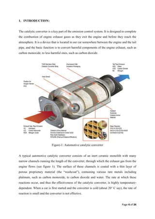
1. 1. INTRODUCTION:
The catalytic converter is a key part of the emission control system. It is designed to complete
the combustion of engine exhaust gases as they exit the engine and before they reach the
atmosphere. It is a device that is located in our car somewhere between the engine and the tail
pipe, and the basic function is to convert harmful components of the engine exhaust, such as
carbon monoxide, to less harmful ones, such as carbon dioxide.
Figure-1: Automotive catalytic converter
A typical automotive catalytic converter consists of an inert ceramic monolith with many
narrow channels running the length of the converter, through which the exhaust gas from the
engine flows (see figure 1). The surface of these channels is coated with a thin layer of
porous proprietary material (the ―washcoat‖), containing various rare metals including
platinum, such as carbon monoxide, to carbon dioxide and water. The rate at which these
reactions occur, and thus the effectiveness of the catalytic converter, is highly temperature-
dependent. When a car is first started and the converter is cold (about 20° C say), the rate of
reaction is small and the converter is not effective.
Page 4 of 34
2. Figure-2: Location of Automotive catalytic converter
As the converter heats up, there is a point somewhere along the converter where the
temperatures first become high enough for significant reaction to occur. At this point, called
the light-off point, the temperature increases dramatically, and this high temperature is
quickly converted downstream by the gas flow. After the light-off point forms, it moves
slowly upstream towards the inlet of the converter as driven by heat diffusion in the solid.
Once the light-off point reaches the inlet, the converter is in full operation.
The warm-up behavior of a catalytic converter is important because it is unable to perform its
task of converting harmful carbon, monoxide and unburnt hydrocarbons to carbon dioxide
and water during this time, due to low converter temperatures. This warm-up period is
relatively short, lasting about 5 minutes or so, but since the duration of many trips in the car
is short, an increased understanding of the behavior of the catalytic converter during its
warm-up period is of obvious importance.
Page 5 of 34
3. 2. MODEL EQUATIONS:
2.1. Facts lying behind the model equations:
a) The chemical reactions in the catalytic converter that take place on the surface of
catalyst. These are exothermic, oxidation reactions involving carbon monoxide,
unburnt hydrocarbons, hydrogen, and oxygen from the exhaust gas.
b) The rate at these chemical reactions occur depends primarily on:
the temperature of the solid converter
the concentration of the reacting species on the surface
The rate of the reactig species are transferred to the catalyst surface from the
gas flow.
small concentrations of nitrogen oxides transferred from the gas and on
irregularities and long-term poisoning of the catalytic surface, among others
c) Heat diffusion in the solid is important but only in the region near the light-off point
where the spatial variation in temperature is large.
d) Heat and mass diffusion in the gas, on the other hand, are not important, because the
residence time for the gas flow is too short.
Figure-3: Catalytic Conversion of Carbon Monoxide and Hydrocarbons
Page 6 of 34
4. 2.2. Mathematical model:
There are a number of references to models of automotive catalytic converters in the
literature, including Heck, Wei, and Katzer [3], Oh and Cavendish [5], Young and Finlayson
[3], [9], and Zygourakis [10].
A useful starting point for the mathematical formulation of a set of model equations, and the
point suggested for this project work, is given by the Oh and Cavendish model.
The Oh and Cavendish model considers the four oxidation reactions [11]:
1
CO O2 CO2
2
9
C 3 H 6 O2 3CO2 3H 2 O
2 (1)
CH 4 2O2 CO2 2 H 2 O
1
H 2 O2 H 2 O
2
Table-1: Typical values for concentrations in the gas[5]
Species Concentrations
CO 2%
C3 H 6 450 ppm
CH 4 50 ppm
H2 0.667%
O2 5%
Figure-4: Individual channel within the monolith.
Page 7 of 34
5. Let consider that,
Species i in the gas. the four oxidands CO , C3 H 6 , CH 4 , and H 2 , indexed by
i
i 1,2,3,4 respectively, and oxygen, i 5
C g ,i The concentration gas of species i in the gas
the corresponding concentration on the surface of the catalyst, where the
C s ,i
reactions are assumed to take place
x the axial distance
t time
ki the mass transfer coefficient of species i
the open frontal area of the converter (the sum of the channel cross-sectional
Ao
areas)
v the average velocity of the gas
P the perimeter of the open area
The equations for the gas are conservation equations. where conservation of mass for species
i in the gas implies the integral form
b b
d b
Ao C g ,i d x Ao vC g ,i a Pki (C s,i C g ,i )
dt a a
(2)
Where,
( a, b ) an arbitrary interval of x
b
d
dt
Ao C g ,i d x the rate of change of mass on the interval ( a, b )
a
b The net flux of mass due to convection across the
b
Ao C g ,i Pk i (C s ,i C g ,i ) boundaries, x a and x b , and the flux of mass to the
a
a
catalyst surface.
The integral form in (2) implies the differential conservation law
C g ,i C g ,i
Ao Ao v Pk i (C s ,i C g ,i ) (3)
t x
In a typical experiment, the velocity is obtained from measurements of the volume flow rate
q . The apparent velocity used in the Oh and Cavendish model is related to q .
Page 8 of 34
6. In a typical experiment, the velocity is obtained from measurements of the volume flow rate
and the average velocity that appears in (2) and (3) by
q Ao v Ac (4)
where,
the apparent gas velocity, which may vary with t due to changeing engine
loads
Ac the frontal area of the converter
By eliminating Ao v in favor of Ac using (4), dividing by Ac , and obtain
C g ,i
t
C g ,i
x
k i S C s ,i C g ,i (5)
where,
A0
the void fraction of the monolith (approximately 0.7)
Ac
P
S the gas-solid surface area per unit volume of converter
Ac
Similar steps involving conservation of heat energy in the gas and obtain
T g
g cg
T g
hS T s T g
(6)
t x
where,
h the heat transfer coefficient
g the dencity of the gas
cg heat capacity of the gas
Ts the temperature of the solid
Tg the temperature of the gas
These two equations (5) and (6) for the gas is called the Oh and Cavendish model equations,
which balance convection with mass and heat transfer to the solid.
Page 9 of 34
7. Assumetion for Oh and Cavendish model: The concentrations and temperatures depend
only on the axial distance and on time, so that these quantities are to be interpreted as cross-
sectional averages.
The Oh and Cavendish model considers the four oxidation reactions (1) with corresponding
reaction rate Ri (i 1,2,3,4; moles per unit time per unit catalyst surface area). Reaction rates
are trypically complicated functions of temperature and concentration involving parameters
chosen to fit experimental data. the precise forms for Ri are given in [5], but these are not
essential for the present discussion.
An approximate form will be discussed in section 3 and used in the subsequent analysis. The
reaction rate is balanced by mass transfer to the catalyst surface so that
a R i (C s , T s ) g ki S (C g ,i C s ,i ) i 1,2,3,4,5 (7)
Where
a The normalized catalyst surface area, which may vary with x due to
design specifications or long-term poisoning
The fifth reaction rate R 5 for oxygen is given by
1 9 1
R5 R1 R 2 2 R 3 R 4 (8)
2 2 2
The final equation in the Oh and Cavendish model:
The final equation in the Oh and Cavendish model comes from conservation of heat
energy in the solid monolith.
It is assumed that the rate of change of heat energy in the solid is balanced by heat
conduction in the solid heat transfer from the gas, and heat production due to
chemical reaction on the surface of the catalyst.
Page 10 of 34
8. An integral form for this balance is given by
b
T s
b b b
d
As s csTs d x As K s x
dt a
Ph(T g T s )d x PQd x
a a
(9)
a
Where
As Ac Ao the solid frontal area of the converter
Ks the thermal conductivity of the solid
Q the rate of heat production per unit gas-solid surface area
s the density of the solid
cs the heat capacity of the solid
The integral form in (9) implies
dTs 2T s
As s c s As K s 2
Ph(T g T s ) PQ (10)
dt x
Assuming that s , c s , and K s are constants. The rate of heat production is given by the sum
of the four oxidation reactions. Thus,
a 4
Q H i R i (C s , T s )
S i 1
(11)
Where
H i 0 is the heat of reaction for species i (heat energy per mole).
The final equation in the model is found by substituting (11) into (10) and dividing by Ac to
give
dTs 2T s 4
1 s cs 1 K s 2
Sh(T g T s ) a H i R i (C s , T s ) (12)
dt x i 1
Page 11 of 34
9. The equation given in (5), (6), (7), and (12) from a complete set or the five species
concentrations and temperature of the gas and the corresponnding concentrations on the
catalyst and the temperature of the solid.
These equations are to be solved for x between 0 and L 10 cm is the length of the
converter, and for t 0 subject to various initial conditions and boundary conditions.
3. SINGLE-OXIDAND MODEL AND NONDIMENSIONALIZATION:
3.1. Assumtion:
a) Consider the behavior of a single generic oxidand, which can be regarded as
carbon monoxide since it is the most abundant pollutant and the dominant heat
source in the system.
b) The concentrations of the remaining oxidands are neglected and thus the
number of equations and complexity of the reaction law is reduced.
c) Under normal conditions, there is a surplus of oxygen in the system which
suggests a further simplification of a constant oxygen concentration.
These simplifications lead to the following set of equations:
C g
t
C g
x
kS C s C g (13)
T g
g cg
T g
hS T s T g
(14)
t x
a R(C s , T s ) g kS(C g C s ) (15)
dTs 2T s
1 s cs 1 K s 2
Sh(T g T s ) a H R(C s , T s ) (16)
dt x
Where
Cg the concentrations of the oxidand in the gas
Cs the concentrations of the oxidand on the surface of the catalyst
Page 12 of 34
10. For the purposes of the analysis, all parameters in the equations will be regarded as constant-
except for , which will be allowed to vary with t , and a with be allowed to vary with x .
Further reductions and simplifications can be made by considering a suitable nondimensional
form for the equations in (13)-(16). Let
x
x
L
t
t
t ref
Cg
Cg
C g ,in
Cs
Cs
C s ,in
T g T g ,in
Tg
T
T s T s ,in
Ts
T
Where
C g ,in 0.02 the oxidand concentration at the inlet of the converter, x 0
T g ,in 300C the gas temperature at the inlet of the converter, x 0
T s ,in the solid temperature at the inlet of the converter, x 0
t ref the reference time
Obvious reference scales have been chosen for distance and concentration. Where are several
choices available for the reference time t ref , but an appropriate one for a study of the warm-
up behavior is given by substituting (14) into (16) and balancing the temperature gradient
dTg
due to heat transfer to the solid with the time-derivative term 1 s cs
dTs
g cg .
dt dt
This choice gives
1 s cs L
t ref 14 sec
g c g ref
Page 13 of 34
11. Where ref 10 m/sec is a chosen reference value for the gas velocity. An appropriate
choice for the reference temperature change is given by
H C g ,in
T 300 C
cg
Which is the temperature increase of the gas stream that would result from a complete
reaction of all of the available oxidand. Using the dimensionless variables in (13)-(16) gives
the following set of dimensionless equations:
C g C g
C s C g (17)
t x
Tg Tg
(Ts Tg ) (18)
t x
aR(Cs , Ts ) C g Cs (19)
dTs 2T
2s (Tg Ts ) aR(C s , Ts ) (20)
dt x
Where the dimensionless gas velocity, normalized catalyst surface area, and reaction rate are
given by
ref
a
a
a ref
a reg R
R
s kSC g ,in
cm 2
a ref 300 is a chosen reference value for the catalyst surface area per unit converter
cm 3
volume, and the four dimensioless paramaters , , , and are given by
kSL Where,
ref
The dimensionless mass transfer coefficients and O(1)
hSL
s cs ref The dimensionless heat transfer coefficients and O(1)
(1 ) K s
The dimensionless solid diffusivity and small
g c g ref
L L
The ratio of the convection time and t ref & very small
ref t ref ref
Page 14 of 34
12. Table-2: Parameter Values
Parameter Values Parameter Values
3 A 0.35
3 Ts ,cold -1
0.001 Tg ,in -0.05
0.0005 C g ,in 1
10
The values for and listed in table-2 are estimates based on discussions with the
industrial representative, because the values for the mass and heat transfer coefficients used
in the Oh and Cavendish model are not reported in [5] The dimensionless solid diffusivity
is small, which indicates that heat diffusion is negligible over the time scale of interest except
in regions where the gradient of the solid temperature is large. This occurs in a small region
(boundary layer) about the light-off point and will be exploited in the later analysis. The last
L
of the four parameters , is the ratio of the convection time and the chosen reference
ref
time. This parameter is very small, indicating that the time-derivative terms in (17) and (18)
may be regarded as negligible.
The reaction rates discussed in [5] are rapidly varying functions of the solid temperature.
When the temperature is low (Ts 0) , the reaction rate is exponentially small, while at a
certain temperature, called the ignition temperature, the reaction rate increases sharply. For
the oxidation of carbon monoxide, this ignition temperature is close to the inlet
temperature (Ts 0) . The reaction rate is also proportional to the surface concentration, so
that the reaction turns off once the oxidand is depleted. In order to keep the analysis as simple
as possible and yet still retain this basic behavior, let us consider a dimensionless reaction
rate given by
RC s , Ts
A
C s e Ts (21)
Where and A are constants. In this form, can be regarded as a dimensionless activation
energy which is typically a large value and A is an O(1) dimensionless rate constant.
Representative values for and A obtained by a rough match with the rate function given in
Page 15 of 34
13. [5] are included in table-2. For large , the reaction behaves like a switch about
Ts Ts ,step 0 (the dimensionless ignition temperature). When Ts Ts ,step the temperature is
low and R 0 , and when Ts Ts ,step , the temperature is high and R is exponentially large
which forces C s 0 according to (19).
Initial and boundary conditions are needed to complete the problem for mulation for the
single-oxidand model. At t 0 , the converter is cold so that –
Ts x,0 Ts ,cold
At the inlet, x 0 , the concentration of oxidand in the gas and its temperature are specified
by the boundary conditions
C g 0, t C g ,in and Tg (0, t ) Tg ,in
Finally, boundary conditions are needed for the solid temperature at both ends of the
converter. Generally there would be some heat flow to the surrounding environment, but for
the-timescale considered the diffusion is negligible so that the no-heat-flux boundary
conditions
Ts
0, t Ts 1, t 0
x x
are a good approximation. Values for Ts ,cold , C g ,in and Tg ,in are listed in table-2.
4. ASYMPTOTIC ANALYSIS OF THE SINGLE-OXIDAND MODEL:
The dynamic behavior of a catalytic converter from a cold start to full operation has two
distinct phases. In the first phase, which will be called warm-up, the converter gently heats up
on an O(1) timescale due mainly to heat transfer from the hot exhaust gas to the solid. Heat
production due to chemical reaction is small during this phase until the solid temperature
reaches the ignition temperature and light-off occurs at some point along the length of the
converter. This event signals the end of the first phase and beginning of the second, which
Page 16 of 34
14. will be called light-off. Once light-off occurs, there is a rapid increase in solid temperature
downstream of the initial light-off point, followed by a slow propagation of the light-off point
1
upstream to the inlet. The second phase, which occurs on an O( 2
) time scale, ends when
the light-off point reaches the inlet and the converter is in full operation.
For the single-oxidand model, asymptotic approximations can be made to study the solution
behavior during each of the two phases. A full solution requires a numerical treatment of the
equation which will be discussed in the next section.
4.1. WARM-UP BEHAVIOR:
During the warm-up phase there are no rapid spatial variations in the solid temperature, so
that heat diffusion in the solid is negligible and the model equation in (17)—(20) reduce to
C g
C s C g (22)
x
Tg
(Ts Tg ) (23)
x
aR(Cs , Ts ) C g Cs (24)
dTs
(Tg Ts ) aR(C s , Ts ) (25)
dt
Where the reaction rate is given in (21) and the initial conditions and boundary conditions are
C g 0, t C g ,in
Tg (0, t ) Tg ,in
Ts x,0 Ts ,cold
Since heat diffusion in the solid is neglected, the boundary conditions on the solid
temperature are not needed. The model equations are still too difficult for analytical progress;
however, one can get a qualitative picture of the solution by making further approximations.
Page 17 of 34
15. Early in the warm-up phase, Ts Ts ,cold so that R is exponentially small. This implies that
C s C g according to (24) and that C s C g ,in according to (22). Further, if Ts Ts ,cold and if
is taken to be constant, then (23) can be integrated to give
x
Tg Ts ,cold Tg ,in Ts ,cold e
(26)
Which shows a decrease in gas temperature with increasing x as expected. As time passes,
Ts increases from Ts ,cold due to heat transfer from the hot exhaust gas until the temperature is
sufficiently large for the chemical reaction to become significant. To study this behavior
qualitatively, let us consider (25) with a known heat source Bx due to heat transfer. Further
let us suppose that C s C g ,in , so that a model problem for Ts is
Ts aAC g ,in Ts
B
e ,
Ts x,0 Ts ,cold (27)
t
The solution for Ts can be written implicitly in the form
Ts Ts ,cold 1 B e TS
t ln (28)
B B B e TS ,cold
Where aAC g ,in .
An example of the behavior of the solution is shown in figure-5. The blowup in the solution
curve occurs when t t b , where
Ts ,cold 1
tb ln TS , cold
(29)
B B B e
Such finite-time blowup (often referred to as thermal runaway) is a common feature of
systems with an exponential heat source. A similar rapid increase in Ts , occurs in the solution
of the equations given in (22)-( 25) and signals the onset of light-off. The main difference is
Page 18 of 34
16. that a constant surface concentration of oxidand is assumed in (27) while in (22)-(25) the
solution curve for Ts , would reach a plateau once the surface concentration is depleted and
the reaction turns off
Figure-5: Behavior of Ts versus time t during the warm-up phase by (7.25) with B 1 . The
blowup time is t b 1.225
4.2. LIGHT-OFF BEHAVIOR:
1
The light-off phase is characterized by an O( 2
) timescale progression of the light-off point
towards the inlet of the converter. On either side of the light-off point, heat diffusion is
negligible, and the solution has reached a steady state (on the timescale of the slow motion)
so that the relevant equations for the outer solution are given by the warm up phase equations
(22)-(25) with the time-derivative term in (25) set to zero. An inner solution connects the cold
solid temperature upstream of the light-off point with the hot temperature downstream. The
solid temperature changes rapidly across this small region, so that heat diffusion becomes
important, and the slow upstream motion of the light-off point.
Page 19 of 34
17. The analysis of this phase proceeds by first considering the Steady-state solution of the
equations in (22)-(25). These equations are
C g
C s C g (30)
x
Tg
(Ts Tg ) (31)
x
aR(Cs , Ts ) C g Cs (32)
0 (Tg Ts ) aR(C s , Ts ) (33)
Where the gas velocity is taken to be constant (or at most slowly varying). At steady state,
heat transfer to the solid balances the reaction rate so that
C g Tg
C s C g Ts Tg 0 (34)
x x
Which implies that,
C g Tg C g ,in Tg ,in (35)
The problem reduces to solving the differential equation for C g or Tg subject to an inlet
boundary condition and the various algebraic equations.
Let us concentrate on the behavior of C g . Since
C g
(C s C g ) aR(C s , Ts ) 0 (36)
x
It is clear that C g is a decreasing function of x . Further, (32) with the reaction rate in (21)
gives
Cg
Cs (37)
aA
1 e Ts
Page 20 of 34
18. Which can be used in (29) with (30) to give
aA Ts
(C g ,in Tg ,in )1
e
Cg (38)
aA aA
1 e Ts
e Ts
Figure-6: Steady-state behavior of Ts versus C g as given by (38)
The curve of Ts versus C g as given by (38) have the shape of a backward S , and the portion
of this curve near C g ,in 1 is illustrated in figure-6. (Note that the curves at the top and
bottom are connected by a lobe of the S curve which is not shown in the figure.) The
solution for C g must lie on this S curve, and the arrows indicate the path from x 0
to x 1. Upstream of the light-off point, C g decreases along the curve from C g ,in on which
Ts is cold. At a point labeled C g , jump , the curve folds back on itself and the path must jump
from the cold temperature at Ts ,turn to a value on the curve where Ts is hot. The solution path
continues with hot values of Ts until x 1. The outer solution consists of the portion of the
Page 21 of 34
19. curve on the cold branch, with C g C g , jump , and the portion of the curve on the hot branch
with C g C g , jump .
It is conjectured that the initial light-off point occurs at the value of x with C g C g , jump as
indicated in figure-6. As time precedes the value of C g , jump increases slowly until the light-off
point reaches the inlet and C g , jump C g ,in (While it has not been shown that the initial jump
must occur at C g , jump and not sooner, the numerical evidence reported in [6] supports this
conjecture.)
The speed of the light-off point is found by considering an inner problem in a small region
about its position, x st , where
C g C g , jump o(1) and Tg Tg ,in C g ,in C g , jump o(1)
In the limit 0 . In this region, diffusion is important, and the full equation for Ts in (20)
must be considered. Using the scaled variables
x st
1
1
and t 2
2
The equation for Ts becomes
ds T 2Ts
(C g ,in Tg ,in C g , jump Ts ) (C g , jump C s ) (39)
d 2
To leading order, where C s , given in terms of Ts by (37) with C g C g , jump . For a given
ds
value of C g , jump , the speed of the light-off point, , is found by insisting that the solution to
d
(39) matches with the correct values of Ts , in the outer solution as .
Page 22 of 34
20. It is instructive to view the inner problem in the phase plane. Let us consider a fixed position
of the light-off point and a corresponding value of C g , jump from the outer solution. The
equations in (39) can be written as the system
Ts' U
' (40)
U U S Ts
where
Ts
U
ds
d
S Ts (C g ,in Tg ,in C g , jump Ts ) (C g , jump C s )
and the primes denote differentiation with respect to the equilibrium points occur when
U 0 and S Ts 0 . There are three equilibrium values of Ts corresponding to the three
intersections of the curve in figure-4 for a given value of C g , jump . Let us label these values
Ts ,1 Ts , 2 Ts ,3 . The equilibrium points at (Ts ,1 ,0) and (Ts ,3 ,0) are saddle points, while
(Ts , 2 ,0) is an unstable node. The correct solution of the inner problem corresponds to the
trajectory in the phase plane that joins the two saddle points. The problem is to find the value
of (an eigenvalue) such that this trajectory exists. The solution of this eigenvalue problem
must be determined numerically, and this will be discussed in the next section.
5. NUMERICAL METHODS AND RESULTS:
A further study of the single-oxidand model can be made by considering numerical methods.
In this section, a numerical treatment of the single-oxidand model is discussed and a solution
to these equations is found. This solution illustrates the warm-up and light-off behaviors
discussed previously and can be used to determine the speed of the light-off point. The speed
of the light-off point as a function of its position can also be found by a numerical solution of
the asymptotic equations in the limit of small , and this result can be compared with the
speed found from the numerical solution of the full set of equations given in (l7)-(20) (with
taken to be zero).
Page 23 of 34
21. The equations for the single-oxidand model are given in (15)-(18) with taken to be zero.
Equations (17), (18), and (19) describe the spatial behavior of C g , Tg and C s respectively,
with the dependence on t given parametrically so that, if Ts is known at a given time, then
solutions for C g , Tg and C s can be found approximately by a numerical integration from the
inlet at x 0 to x 1. For example, using (19) and (21) in (17) gives
aA Ts
e
C g
C g , with C g (0, t ) C g ,in (41)
x
1 aA e Ts
For later convenience, define
aA Ts
e
K Ts , x
1 aA e Ts
If Ts is regarded as a known function of x and t , the solution to (41) is
x
0
K (Ts , x ' )dx'
Cg Cg ,ine
(42)
Likewise, (18) can be integrated to give
x '
x x'
x
Tg Tg ,in e
Ts e
dx ' (43)
0
The integrals in (42) and (43) can be evaluated numerically. Let C g , j , and Tg , j approximate
1
C g and Tg , respectively, at grid x j jh , j 0,1,...., N where h for a chosen integer
N
N (the total number of grid cells).
Page 24 of 34
22. Second-order accurate approximations for (42) and (43) are given by the iteration
h
K ( Ts , j , x 1 )
j
2
Cg , j Cg , j 1e
, with C g ,o C g ,in (44)
and
h ' h
Tg , j Tg , j 1e 1 e ,
Ts , j with Tg , o Tg ,in (45)
1
Respectively, where j 1,2,...., N and Ts , j approximates Ts at the cell center j h .
2
The time evolution of the solid temperature on the grid is given by the ordinary differential
equations
dTs , j T 2Ts , j Ts , j 1 ^ ^
s , j 1
T g , j Ts , j K Ts , j , x 1 C g , j
(46)
h2 j
dt 2
For j 1,2,...., N where
Cg , j Cg , j 1
^ 1
C g, j
2
T g , j Tg , j Tg , j 1
^
1
2
Ts ,1 Ts , 0
Ts , N 1 Ts , N
Which represent a second-order accurate approximation of the evolution equation for Ts in
(20). In view of (44) and (45), the system of equations in (46) has the form
dT s
F (T s , t ) (47)
dt
Where T s is a vector with components Ts , j , j 1,2,...., N . The initial conditions for this
system are given by Ts , j Ts , cold There are many standard numerical techniques available for
Page 25 of 34
23. integrating (47). The choice used here is the midpoint rule, which is a second-order-accurate
Runge-Kutta method.
Figure-7: Numerical solution for the single-oxidand model. The arrows indicate the
progression of time from t 0 to t 24( 5.6 min) . The interval of time between successive
curves is 0.8( 11.2 sec)
A numerical solution for the choice of parameters in table -2 is shown in figure -7. For this
solution, it is assumed that the catalyst surface area ax and gas velocity t are constant
and both taken to be 1, although those functions could be allowed to vary without difficulty
for the numerical method. The behaviors of Cs and Ts at successive times are shown in
figures 7(a) and 7(b), respectively. The arrows in the figures indicate the progression of time.
During the warm-up phase, the solid temperature is relatively cold(less than zero) and the
Page 26 of 34
24. reaction rate is negligible, so that the surface concentration of oxidand is approximately equal
to the gas concentration, which, in turn, is nearly equal the inlet value Cg ,in 1 . Near the end
of the warm-up phase, the solid temperature approaches the ignition temperature, so that the
rate of reaction becomes significant. The onset of light-off and the subsequent motion of the
light-off point can be seen most clearly in the plot of Cs as the large reaction rate forces the
surface concentration to zero. The solid temperature rises at the light-off point over a small
1
O 2 distance, as predicted by the previous asymptotic analysis. As time proceeds, this
1
light-off point moves slowly (on an O 2 time scale) towards the inlet. The behaviors of
C g and Tg are shown in figures 7(c) and 7(d) respectively, and these curves also illustrate the
predicted behaviors.
1
ds
The speed of the light-off point 2 can be found by solving the eigenvalue problem
dt
for as given by the system of equations in (40). The system of equations can be reduced to
the first-order ODE.
dU S Ts
(48)
dTs U
with boundary conditions U Ts ,1 U Ts ,3 0 for a given value of C g , jump , this eigenvalue
problem can be solved numerically using a shooting approach. The idea is to solve (48) for
Ts Ts ,1 using the left boundary condition and separately for Ts Ts ,3 using the right
boundary condition. These solutions can be found numerically using a provisional choice for
. At the intermediate point, Ts
1
Ts,1 Ts,3 , the values of U for the two solutions would
2
not agree in general, and a method of iteration (Newton’s method) is used to find the correct
value of which produces agreement at this point from both side.
Once is found for a given value of C g , jump , the remaining problem is to connect the light-
off position s to the corresponding value of C g , jump . This can be done by returning to the
Page 27 of 34
25. steady-state outer equations in (30)-(33) and integration the ODE for C g from x 0 , where
Cg Cg ,in , to x s , where Cg Cg , jump . For each value of s, a corresponding value C g , jump is
1
ds
found, which, in turn, implies a value for 2 , from the solution of the eigenvalue
dt
problem. The curve in figure-8 shows the speed of the light-off point as a function of its
position for the case when 0.001 . The data points in this figure show the speed of the
light-off point as determined from the numerical solution of the full equations given in figure-
7. Good agreement is noted (and expected since is small) except near the inlet, where the
asymptotic solution is not valid, and for larger s , where there is some difficulty in identifying
the light-off position as it is forming in the numerical solution.
ds
Figure-8: Light-off point speed versus position s
dt
6. FURTHER ANALYSIS OF THE SINGLE-OXIDAND MODEL
The analysis discussed in section 4 considered the small diffusion limit, 0 , which
revealed the two-phase structure of the solution and the boundary layer behavior near the
light-off point. Analytical solutions of the reduced equations for each phase are not available
Page 28 of 34
26. (although a numerical treatment of these equations is fairly straightforward) mainly due to the
nonlinear reaction term which remains in these equations in its original form. In order to
make further analytical progress, there needs to be some approximate treatment of the
reaction term. This can be done by appealing to an asymptotic analysis of the equations in the
limit of large activation energy, which implies the limit for the present reaction
model. Pursuing this line of approach reveals even more structure of the equations and gives
some analytical results, including an estimate for the initial position of the light-off point and
a formula for the light-off point speed.
From a mathematical view, it is interesting to look at this limiting case, but in the end there
will be some concern over its validity, because the large parameter in question is only 10
according to value given in table-1. For this reason, only a brief discussion of these results is
presented here. The interested reader can find the full details in [6] or work them out
independently.
An estimate for the initial light-off point comes from an analysis of the cold branch of the
1
curve in figure 6. In the limit of large activation energy, it is assumed that Ts O on this
branch, so that (38) reduces to
A*
C g C g ,in Tg ,in Ts e Ts (49)
where
A* C g ,in Tg ,in aA
At the inlet, C g C g ,in and Ts takes a value, Tg ,in say, corresponding to the smallest solution
of
A* Ts ,in
Ts Tg ,in e
Page 29 of 34
27. It is assumed that the inlet conditions are such that Ts ,in exists on the cold branch; otherwise
the only solution would lie on the hot branch of figure-4, and the initial light-off point would
occur at the inlet. According to the reduced form in (49), a value for Ts ,turn is given by
1
Ts ,turn ln A*
dC g
Which corresponds to the point where 0 . The values of x on this branch are
dTs
determined from (30) which, using (49), reduces to solving
A* T
1 A*e T s
T
s
e s
x
with Ts Ts ,in at x 0 . The solution is
1 Ts A* 1 T
e A Ts
*
x e A*Ts ,in
s , in
The initial light-off point, x s0 say, occurs when Ts Ts ,tirn , which gives the estimate
1 T
s0 ln A 1 Ts ,in * e
* s , in
A
It is interesting to note that, if the inlet conditions are such that s0 1 , then the system would
be too cold for light-off to occur.
An estimate for the speed of the light-off point can be found by considering the eigenvalue
problem given by
C g ,in Tg ,in C g , jump Ts C g , jump Cs
ds dTs d 2Ts
(50)
d d d 2
Page 30 of 34
28. In the limit .The value of C s is given by (37) with C g C g , jump . The simplest analysis
of this problem replaces (37) by the step function
C g C g , jump H Ts ,step Ts (51)
Where H is the Heaviside function and Ts ,step is the ignition temperature. This approximation
has the correct behavior away from the light-off point and would give the correct speed for
the some value of Ts ,step While it is not known what the correct value is, a reasonable choice
is
1 aA
Ts ,step ln
Which corresponds to the value where the reaction rate changes most rapidly. This chase is
used in [6] and suggested by the work of [1] and [4]. It is straightforward to solve the linear
equation in (50) with C s given by (51) for Ts on either side of Ts ,step and then join the
solutions at Ts ,step . This result in an estimate for the light-off point Speed given by
ds C g , jump 2
d
C g , jump
1 1
2 2
Where Ts ,step Tg ,in C g , jump C g ,in
Which reduces to
1
ds C g , jump 2
(52)
d
upon noting that is small and positive and C g , jump O(1)
A formal asymptotic analysis can be made of the equation in (50) and (37) without the use of
the step-function approximation. The structure of the solution is more complicated than the
previous analysis. Four regions emerge with appropriate scalings of and Ts for each. A
solution can be found for the relevant equations in each region and then matched with the
Page 31 of 34
29. solutions on either side. Details are given in [6]. In the end, the analysis yields a formula for
the light-off point speed which agrees to leading order with the one given by (52).
The estimates for the initial position of the light-off point and its speed can be checked by
comparing these results with the numerical solution of the equations. This is done in [6], and
it is found that the estimate for the initial light-off position is in good agreement with the
numerical results, while the speed of the light-off point is not. The asymptotic expansion for
ds 1
the involves powers of the ―small parameter‖ 0.43 , which is not very small, and
d ln
would suggest poor accuracy for an estimate using only the leading terms in the expansion.
7. CONCLUDING REMARKS
A detailed asymptotic and numerical treatment has been given for the single-oxidand model
with the aim of answering the questions posed by the industrial representative. Let us review
these questions briefly and summarize the results that have been obtained. The first question
concerned the formulation of a reduced model suitable for analysis. This question has been
answered with the formulation of the single-oxidand model. This model is significantly
simpler than the original Oh and Cavendish model and yet retains the essential features of the
more complicated model. The second question involved an analysis of the reduced model and
a search for analytical solutions to study the warm-up period of the converter’s operation. An
analysis of the reduced model in the limits of small diffusion revealed a two-phase structure
during the warm-up period. The timescale for the first (warm-up) phase was found to be
O t ref while the timescale for the second (light-off) phase was found to be much slower. The
1
timescale for the latter phase was found to be O 2 t ref
. A good understanding of the
solution was obtained analytically for each phase but a numerical method was needed to find
the quantitatively. A relatively simple numerical method was found for the reduced model.
This numerical method was used to verify analytical result, but could also be used to find
solutions for varying running conditions or for a variety of parameter values in answer to the
last question posed by the industrial representative.
Page 32 of 34
30. The work presented here can be extended in various ways. For example, the simple reaction
given in (21) for the reduced model could be replaced by one that includes the effects of
oxygen depletion and nitrogen oxide inhibition. This extension brings the reaction rate model
closer to the more complicated forms given in [5] and would require additional equations for
the gas and surface concentrations of oxygen. The concentration of nitrogen oxides is small
and could be taken to be constant. This extension is discussed in [6]. A further extension,
discussed in [7] following the work in [10], considers a two-dimensional model that includes
radial variations in the converter cross-section due to nonuniformities in gas velocity and
solid temperature. A fairly straightforward modification of the numerical method discussed
here could be used to study these radial variations.
8. REFERENCES:
[1] Byme, H. & Norbury, J. (1990) Catalytic converters and porous medium
combustion. In Emerging Applications in Free Boundary Problems, proc. 5th
International Colloquium on Free Boundary Problems (eds. Chadam, J.M. &
Rasmussen, H.) Montreal, Canada, May 1990.
[2] Hagan, P. S., King, J. R., Nelligan, J. D., Please, C. P. & Schwendeman, D. W.
(1989) Dynamic behavior of automotive catalytic converters. In Proc. 5th RP1
Workshop on Mathematical Problems in Industry, Troy, New York. USA.
[3] Heck, R. H., Wei, J. & Katzer, J . R. (1976) Mathematical modeling of monolithic
catalysts. AIChE J. 22, 477-484.
[4] Norbury. I. & Stuart, A. M. (1989) Models for porous medium combustion. Quart.
J. Mech. Appl. Math. 42, 159-178.
[5] Oh, S. H. 8: Cavendish, J. C. (1982) Transients of monolithic catalytic converters:
Response to step changes in feed-stream temperature as related to controlling
automotive emissions. Ind. Chem. Prod. Res. Dev. 21. 29-37.
[6] Please, C. P., Hagan P. S. & Schwendeman D W (1994) Light-off behavior of
catalytic converters. SIAM J. Appl. Math. 54, 72-92.
[7] Ward, J. P. (1991) Mathematical modeling of the dynamics of monolithic catalytic
converters for the control of automotive emissions, Mathematics and Computer
Science Final-Year Project, University of Southampton, England.
Page 33 of 34
31. [8] Young, L. C. & Finlayson, B. A. (1976) Mathematical models of the monolith
catalytic converter: Part I. Development of model and application of orthogonal
collocation. AIChE J. 22, 331-343.
[9] Young, L. C. & Finlayson, B. A. (1976) Mathematical models of the monolith
catalytic converter: Part II. Application to automobile exhaust. AIChE J. 22, 343--
353.
[10] Zygourakis, K. (1989) Transient operation of monolith catalytic converters: A
two-dimensional reactor model and the effects of radially nonuniform flow
distributions. Chem. Eng. Sci. 44, 2075-2086.
[11] Ellis Cumberbatch and Alistair Fitt (2001). Mathematical Modeling: Case Studies
from Industry. Cambridge University Prass, UK, 135-159.
[12] Impens, R., ―Automotive Traffic: Risks for the Environment‖, Stud. Surf. Sc.
Catal. 30, 11-30, 1987.
[13] Mabilon, G., Durand, D. and Courty, Ph., ―Inhibition of Post-Combustion
Catalysts by Alkynes: A Clue for Understanding their Behaviour under Real
Exhaust Conditions‖, Stud. Surf. Catal. 96, 775-788, 1995.
[14] M. Balenovic, J. H. B. J. Hoebink and A. C. P. M. Backx, and A. J. L. Nievergeld.
“Modeling of an Automotive Exhaust Gas Converter at Low Temperatures
Aiming at Control Application”, Society of Automotive Engineers, Inc.1999.
Page 34 of 34