Selected Problem solutions from Ch5 (Image recontruction and restoration) Digital Image Processing 3E by Gonzalez and woods

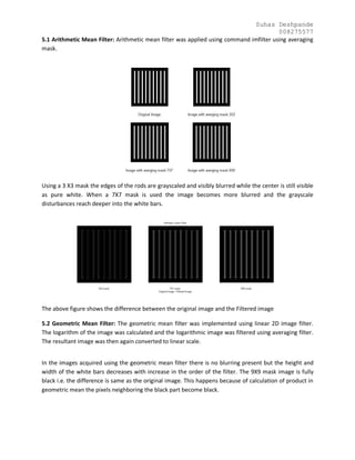
1. Suhas Deshpande
008275577
5.1 Arithmetic Mean Filter: Arithmetic mean filter was applied using command imfilter using averaging
mask.
Using a 3 X3 mask the edges of the rods are grayscaled and visibly blurred while the center is still visible
as pure white. When a 7X7 mask is used the image becomes more blurred and the grayscale
disturbances reach deeper into the white bars.
The above figure shows the difference between the original image and the Filtered image
5.2 Geometric Mean Filter: The geometric mean filter was implemented using linear 2D image filter.
The logarithm of the image was calculated and the logarithmic image was filtered using averaging filter.
The resultant image was then again converted to linear scale.
In the images acquired using the geometric mean filter there is no blurring present but the height and
width of the white bars decreases with increase in the order of the filter. The 9X9 mask image is fully
black i.e. the difference is same as the original image. This happens because of calculation of product in
geometric mean the pixels neighboring the black part become black.

2. Suhas Deshpande
008275577
The above figure shows the difference between the Original image and filtered image. The 3X3 mask
removes the outer edge of the rods which shows out as white after subtraction. The edge deepens in
the case of 7X7 mask and covers the whole rod in 9X9 mask. Thus the 9X9 mask image is black.
5.3 Harmonic Mean Filter: Harmonic mean filter was implemented using the formula
i.e. Averaging filter was applied to the image with reciprocal of each pixel value and the result was again
inversed.
After the Harmonic mean filter the rods in the image are reduced in width but we can se less or no
reduction in the width of 2nd 5th and 8th rod for 3X3 mask image. That may be because the mask size. the
bars is 7X7 masked image are much more thinned and finally for the 9X9 mask the rods disappear. the
rods disappear due to overlapping of the masked regions. The distance between the rods is 17 pixels
and there is overlapping.

3. Suhas Deshpande
008275577
The above image shows the difference image between the original image and the filtered image.
5.4 Contra-Harmonic Mean Filter: The contra-harmonic mean filter was applied by taking the ratio of
two averaging filters one with each pixel squared and other the original image.
The contra-harmonic mean filtered image is similar to the harmonic mean filter but the rods increase in
width on the contrary to the harmonic mean filter.

4. Suhas Deshpande
008275577
The above image shows the difference between the filtered image and original image. We can see the
extra pixels which are white in filtered image than the original image.
5.6 Median Filter: To implement the median filter the command used is medfilter2
The median filter affects and blurs out the corners of the white bars i.e the area with ¼ th of 1s (white)
and 3/4th of 0s (black). This happens because at the edges the median is equal to 0 as the number of 0s
greater than number of 1s.

5. Suhas Deshpande
008275577
The difference image shows the white spots at the edges of the rods. The spots become larger as the
size of mask is increased.
5.7 Max Filter: Max filter was implemented using ordfilt2.
In the image filtered using the max filtered width and height increases more than any other filter. There
will be increase in n-1 pixels where n is the order of the mask.
The above figure shows the difference between the filtered image and original image. The added white
pixels in the filtered image can be seen. The white pixels added around the bars increase with increase
in order of the mask.
5.10
In Arithmetic mean filter the image gets blurred because the pixel value is calculated by as an average of
the neighboring pixels. Similarly in geometric mean filter the pixel value is calculated as the 1/n th
power of the product of the neighboring pixels. Thus at the edge where 0s and 1s are adjacent to each

6. Suhas Deshpande
008275577
other in a binary image (High frequency points), the image gets blurred in the case of arithmetic mean
filter and the image is black for the geometric mean filter. Because of product calculation the pixels
neighboring a 0 automatically become 0 in geometric mean filter and instead of blurring be see an
extended ‘0’ (black) area.
For this reason the black bars are wider in geometric filtered image.
5.11 The contra-harmonic filter is given by
a) Pepper noise is nothing but black spots (noise) all over the image. In image spacial domain
these are zeros. When Q is positive numerator is greater than the denominator thus the transfer
function is greater than 1. Thus the low intensity pixels are affected i.e. the zeros or the ‘pepper’
is removed. This is because for a pixel with intensity 0 or near zero the contra-harmonic mean of
pixels around it is much greater than zero i.e. not a ‘pepper’.
b) Salt noise is nothing but white spots all over the image. In spacial domain these are valued the
high intensity pixels. When Q is negative the numerator is less than the denominator thus the
transfer function is less than 1. Thus the high intensity pixels are affected i.e. the zeros or the
‘pepper’ is removed. This is because for a pixel with high intensity (255 or near 255) the contra-
harmonic mean of pixels around it is much lesser than 255 i.e. not a ‘pepper’.
c) When Q < 1 is chosen for pepper noise more dark spots are created. The noise level increases.
Similarly when Q > 1 is chosen for the salt noise more white spots are created . The noise level
increases again.
d) For Q =-1
When we choose Q = -1 we see that the equation for the contra-harmonic filter reduces to
harmonic mean filter, which works well to filter salt noise as it reduced the intensity of the noisy
pixels. It also works fine for Gaussian noise.
e) The contra-harmonic filter does not affect the constant intensity regions in an image. This is
because the contra-harmonic mean of ‘n’ numbers with value ‘x’
CHmean =
Thus the pixel intensity does not change if a contra-harmonic mean filter is applied to an image
with constant intensity.

7. Suhas Deshpande
008275577
Result Images
5.1 Image filtered using Averaging filter 5.2 Image filtered using Geometric Mean Filter
5.3 Image Filtered Using Harmonic Mean Filter 5.4 Image Filtered Using Contra-Harmonic Mean Filter
5.6 Image filtered using Median Filter 5.7 Image filtered using max Filter

8. Suhas Deshpande
008275577
Matlab codes:
%% Figure for problem 5.1 %%
bars = ones(210,7);
gaps = zeros(210,17);
I1 = [bars gaps];
I = [repmat(I1,1,8),bars];
[m,n] = size(I);
mb = m+40; nb = n+40;
Ib = zeros(mb,nb);
Ib(21:m+20,21:n+20) = I;
subplot(2,2,1);
imshow(Ib);
xlabel('Original Image');
%% Arithmetic mean %%
% Arithmetic mean 3X3 filter
f1 = fspecial('average', 3);
Iavg3 = imfilter(Ib,f1,'corr');
subplot(2,2,2);
imshow(Iavg3);
xlabel('Image with averging mask 3X3');
% Arithmetic mean 7X7 filter
f2 = fspecial('average', 7);
Iavg7 = imfilter(Ib,f2,'corr');
subplot(2,2,3);
imshow(Iavg7);
xlabel('Image with averging mask 7X7');
% Arithmetic mean 9X9 filter
f3 = fspecial('average', 9);
Iavg9 = imfilter(Ib,f3,'corr');
subplot(2,2,4);
imshow(Iavg9);
xlabel('Image with averging mask 9X9');
%% Geometric Mean %%
%% Geometric Mean using 3X3 mask %%
avg1 = fspecial('average',3);
logI = log(Ib);
Igeo1 = imfilter(logI,avg1,'corr');
Igeo1 = exp(Igeo1);
subplot(2,2,2);
imshow(Igeo1);
xlabel('Image Filtered Using 3X3 Geometric mask');
%% Geometric Mean using 3X3 mask %%
avg2 = fspecial('average',7);
logI = log(Ib);
Igeo2 = imfilter(logI,avg2,'corr');
Igeo2 = exp(Igeo2);
subplot(2,2,3);
imshow(Igeo2);
xlabel('Image Filtered Using 7X7 Geometric mask');
%% Geometric Mean using 3X3 mask %%
avg = fspecial('average',9);

9. Suhas Deshpande
008275577
logI = log(Ib);
Igeo3 = imfilter(logI,avg,'corr');
Igeo3 = exp(Igeo3);
subplot(2,2,4);
imshow(Igeo3);
xlabel('Image Filtered Using 9X9 Geometric mask');
%% Harmonic Mean %%
J = 1./Ib;
% Harmonic mean filter using 3X3 mask %
f1 = fspecial('average',3);
Javg1 = imfilter(J,f1,'corr');
Iharmean1 = 1./Javg1;
subplot(2,2,2);
imshow(Iharmean1);
xlabel('Image filtered using 3X3 Harmonic mask');
% Harmonic mean filter using 7X7 mask %
f2 = fspecial('average',5);
Javg2 = imfilter(J,f2,'corr');
Iharmean2 = 1./Javg2;
subplot(2,2,3);
imshow(Iharmean2);
xlabel('Image filtered using 7X7 Harmonic mask');
% Harmonic mean filter using 9X9 mask %
f3 = fspecial('average',9);
Javg3 = imfilter(J,f3,'corr');
Iharmean3 = 1./Javg3;
subplot(2,2,4);
imshow(Iharmean3);
xlabel('Image filtered using 9X9 Harmonic mask');
%% ContraHarmonic Mean filter %%
figure;
subplot(2,2,1);
imshow(Ib);
xlabel('Original Image');
I2 = Ib .* Ib;
% Contraharmonic filter using 3X3 mask %
f1 = ones(3);
Num1 = imfilter(I2,f1,'corr');
Den1 = imfilter(Ib,f1,'corr');
Iconharmean1 = Num1./Den1;
subplot(2,2,2);
imshow(Iconharmean1);
xlabel('Image Filtered Using 3X3 Contra-Harmonic mask');
% Contraharmonic filter using 7X7 mask %
f2 = ones(7);
Num2 = imfilter(I2,f2,'corr');
Den2 = imfilter(Ib,f2,'corr');
Iconharmean2 = Num2./Den2;
subplot(2,2,3);

10. Suhas Deshpande
008275577
imshow(Iconharmean2);
xlabel('Image Filtered Using 7X7 Contra-Harmonic mask');
% Contraharmonic filter using 9X9 mask %
f3 = ones(9);
Num3 = imfilter(I2,f3,'corr');
Den3 = imfilter(Ib,f3,'corr');
Iconharmean3 = Num3./Den3;
subplot(2,2,4);
imshow(Iconharmean3);
xlabel('Image Filtered Using 9X9 Contra-Harmonic mask');
%% Median Filter %%
% Median filter using 3X3 mask %
Imed1 = medfilt2(Ib,[3,3]);
subplot(2,2,2);
imshow(Imed1);
xlabel('Image filtered using 3X3 Median mask');
% Median filter using 7X7 mask %
Imed2 = medfilt2(Ib,[7,7]);
subplot(2,2,3);
imshow(Imed2);
xlabel('Image filtered using 7X7 Median mask');
% Median filter using 9X9 mask %
Imed3 = medfilt2(Ib,[9,9]);
subplot(2,2,4);
imshow(Imed3);
xlabel('Image filtered using 9X9 Median mask');
%% Max filter %%
%% Max filter using 3X3 mask %%
Imax1 = maxfilt2(Ib,[3,3]);
subplot(2,2,2);
imshow(Imax1);
xlabel('Image filtered using 3X3 mask');
%% Max filter using 7X7 mask %%
Imax2 = maxfilt2(Ib,[7,7]);
subplot(2,2,3);
imshow(Imax2);
xlabel('Image filtered using 7X7 mask');
%% Max filter using 9X9 mask %%
Imax3 = maxfilt2(Ib,[9,9]);
subplot(2,2,4);
imshow(Imax3);
xlabel('Image filtered 9X9 mask');
%% Max filter %%
% Max filter using 3X3 mask %
Imax1 = ordfilt2(Ib,1,ones(3));
subplot(2,2,2);

11. Suhas Deshpande
008275577
imshow(Imax1);
xlabel('Image filtered using 3X3 mask');
% Max filter using 7X7 mask %
Imax2 = ordfilt2(Ib,1,ones(7));
subplot(2,2,3);
imshow(Imax2);
xlabel('Image filtered using 7X7 mask');
% Max filter using 9X9 mask %
Imax3 = ordfilt2(Ib,1,ones(9));
subplot(2,2,4);
imshow(Imax3);
xlabel('Image filtered 9X9 mask');
%% 5.8 Min Filter %%
figure;
subplot(2,2,1);
imshow(Ib);
xlabel('Original Image');
% Min Filter using 3X3 mask %
Imin1 = ordfilt2(Ib,3*3,ones(3));
subplot(2,2,2);
imshow(Imin1);
xlabel('Image filtered using 3X3 min mask');
% Min Filter using 7X7 mask %
Imin2 = ordfilt2(Ib,7*7,ones(7));;
subplot(2,2,3);
imshow(Imin2);
xlabel('Image filtered using 7X7 min mask');
% Min Filter using 9X9 mask %
Imin3 = ordfilt2(Ib,9*9,ones(9));
subplot(2,2,4);
imshow(Imin3);
xlabel('Image filtered 9X9 min mask');