1) The document discusses which seismic attributes are most useful for quantitative seismic reservoir characterization. It analyzes attributes such as zero phase amplitude, relative impedance, and absolute impedance.
2) The conclusion is that an absolute impedance inversion provides the best attribute in theory but is difficult in practice. A relative impedance inversion, which is easier to generate, works nearly as well for characterization.
3) Key advantages of relative impedance over zero phase amplitude include relating to geology rather than just impedance contrasts, and allowing comparison between seismic datasets and well logs after appropriate scaling. However, relative impedance lacks low frequency content included in absolute impedance.
Cloud Frontiers: A Deep Dive into Serverless Spatial Data and FME
Seismic attributes
1. What is the Best Seismic Attribute for Quantitative Seismic Reservoir Characterization?
Dennis Cooke*1, Arcangelo Sena 2, Greg O'Donnell 3 , Tetang Muryanto 4 and Vaughn Ball 4 . 1 ARCO Alaska, 2
ARCO Exploration Technology, 3 ARCO Indonesia, 4 Matador Petroleum formerly ARCO Exploration
Technology
Summary phase data, relative impedance data or absolute impedance
data. In our opinion, these three attributes (zero phase
It is possible to generate at least 30 different seismic amplitude, relative impedance and absolute impedance) are
attributes from a given seismic data set. This presentation the most useful for quantitative reservoir characterization.
addresses the question of which of those post-stack
attributes is most appropriate to use for a quantitative 3)Interval attributes are those that are used to quantify a
seismic reservoir characterization. Our conclusion is that window of seismic data usually containing more than one
an absolute impedance inversion is the best attribute in peak or through. Most seismic attributes fall into this
theory, but, in practice, a relative impedance inversion is category. Examples of interval attributes are number of
much more practical. zero crossings, average energy and dominant frequency.
These attributes are frequently used when a reservoir's
Introduction seismic reflection(s) are so discontinuous that it is
impossible 'pick' the same peak or trough on all traces. An
Reservoir characterization is the process of mapping a interval attribute is analogous to a well log cross section
reservoir's thickness, net-to-gross ratio, pore fluid, porosity, with a number of thin, discontinuous sands that can not be
permeability and water saturation. Traditionally, this has correlated with any certainty. For this reservoir, a net-to-
been done in a field development environment using data gross sand ratio map is made instead of individual sand
from well logs. Within the past few years, it has become (flow) unit thickness maps. A seismic reservoir
possible to make some of these maps using seismic characterization is always improved if all peaks and troughs
attributes when those attributes are calibrated with over the reservoir interval can be 'picked' individually and
available well control. The advantage of using wells and thus have quantitative attributes extracted. If this is not
seismic instead of just wells alone, is that the seismic data possible, the use of interval attributes is warranted.
can be used to interpolate and extrapolate between and
beyond sparse well control. 4)AVO attributes are those that are generated using a
reflection's pre-stack amplitudes. Examples of pre-stack
There is a multitude of different seismic attributes that can attributes are AVO gradient, AVO intercept, near
be generated from a given seismic data set. A quick review amplitude and far amplitude. 3D pre-stack attributes have
of one popular seismic interpretation package shows that only become available recently with the advent of
one can generate at least 30 different seismic attributes affordable pre-stack time migrations. Pre-stack attributes
from an input seismic survey. Some of these attributes are have a lot of promise, but are beyond the scope of this
much better than others for reservoir characterization, but presentation.
there has not been much discussion of this in the
geophysical literature. The objective of this presentation is This talk will focus on the three main quantitative attributes
to try to classify seismic attributes and show which ones (zero phase, relative impedance and absolute impedance)
work best for reservoir characterization. and address their respective advantages and disadvantages.
One way to organize and understand seismic attributes is to Zero Phase Amplitudes
separate them into the following four categories:
All seismic attributes are calculated from the final migrated
1)Qualitative attributes such as coherency - and perhaps zero phase dataset (or what is believed to be zero phase).
instantaneous phase or instantaneous frequency - are very Clearly, the easiest, fastest, least expensive attribute is the
good for highlighting spatial patterns such as faults or zero phase amplitude. The convolutional model and the
facies changes. It is difficult if not impossible to relate reflection coefficient formula show that a reflector's zero
these attributes directly to a logged reservoir property like phase amplitude can be directly related to the reservoir's
porosity or thickness, and thus these attributes are not impedance. A thin-bed tuning curve model shows that zero
normally used to quantify reservoir properties. phase amplitude is also directly related to reservoir
thickness. Additionally, gas substitution modeling shows
2)Quantitative attributes: The simplest quantitative that a reservoir's zero phase amplitude can be influenced by
attributes are the amplitude (of a peak or a trough) on zero changes in pore fluids. A solid theoretical conclusion is that
2. What is the Best Seismic Attribute for Reservoir Characterization?
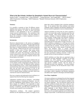
changes in zero phase amplitude are a function of changes oil sand. The cap rock impedance varies due to lateral
in reservoir impedance, thickness and pore fluid. This lithology changes and because it is a waste rock and
conclusion has been proven by many successful contains some oil and/or gas.
quantitative reservoir characterizations done with zero
phase amplitude.
Absolute Impedance and its Advantages
The absolute impedance attribute can be generated with
either a Seislog ® type impedance inversion (one that
includes a low frequency background model) or a model-
based inversion such, as that first described in Cooke and
Schneider (1983). There are two major motivations for
using absolute impedance for reservoir characterization:
1)The amplitudes on an absolute impedance dataset
describe the impedance of the rocks, where the amplitudes
on a zero phase dataset describe the impedance contrast
between rocks. Put another way, the impedance attribute is
related to the geology while the zero phase attribute is Figure2: Reflection coefficient probability distribution.
related to the derivative of the geology. The importance of Calculated using the impedances in Figure 1 and the formula:
this difference can not be overstated for the case where the RC = (Z2-Z1)/(Z2+Z1) where Z1 and Z2 are the impedances of
the cap and reservoir rock.
impedance of both the reservoir and the surrounding rock
are changing laterally. Consider Figure 1 which shows the
2)The second major motivation for using absolute
distribution of impedance for both cap rock and reservoir
impedance instead of zero phase amplitude concerns the
rock (gas filled and oil filled) at Prudhoe Bay Field. These
amplitude scale and format problem that occurs with zero
distributions can be input into the reflection coefficient
phase data. Consider an undrilled gas prospect on one 3D
formula which leads to the reflection coefficient
survey, with a second 3D survey that covers a nearby gas
distributions of Figure 2. Figure 1 corresponds to absolute
discovery. With zero phase seismic data, the prospect's
impedance data and Figure 2 would correspond to zero
amplitudes and the gas discovery's amplitudes can not be
phase data (without a seismic wavelet). Clearly, the ability
compared (unless a similar empirical scaling has been
to discriminate between oil filled reservoir and gas filled
applied to both). Furthermore, the gas discovery's logs can
reservoir is enhanced in the absolute impedance case.
not be compared the amplitudes on the zero phase seismic
data. When both 3Ds are converted to absolute impedance,
the seismic amplitudes can be compared to each other and
to the impedance logs from the gas well.
Disadvantages of Absolute Impedance
Absolute impedance inversions can be very expensive in
terms of both money and time delays. Frequencies in the
inversion above the seismic bandpass will be non-unique.
And since the input zero phase seismic data does not
contain frequencies below the seismic bandpass (which are
required for inversion), information at these frequencies
must be supplied by the processor. The work that is done
to prepare and constrain the low frequency portion of
inversions can be very subjective and interpretive. Most
often, this work on the low frequencies is not done by the
interpreter, but by others who may not communicate to the
Figure 1: Probability density functions for the acoustic impedance interpreter the subjective nature of the low frequencies.
of Sadlerochit reservoir and Shublik cap rock at Prudhoe Bay
Field.
A good way to understand the problem with the low
The data in Figure 1 are taken from a gas well and an oil frequencies in absolute impedance inversion is to consider
well. As expected, the gas sand has slower impedance that a hypothetical inversion between two wells as in Figures
3A and 3B. Wells A and B at structural highs have tight
3. What is the Best Seismic Attribute for Reservoir Characterization?
and thin reservoir (marked in yellow). A prospective
location exists between the wells, but it is not clear if the
reservoir there is better or worse than on the highs (and this
is why the inversion is being done). The inversion process
requires input of a low frequency (below seismic
bandwidth) impedance for all traces. At wells A and B,
this low frequency is taken from the well control. At all
other locations, the processor must interpolate, interpret or
guess at this low frequency input. At the proposed
location, this low frequency guess could take the form of a
linear interpolation between wells A and B (shown in black
in 3A). Alternatively, the low frequencies at this location
could be modified to fit the structure of the reservoir (i.e.
shifted down to tie the yellow horizon). Additionally, the
low frequency input could be modified to fit hypothetical Figure 3A. Hypothetical inversion example.
depositional models. Two possible depositional models:
Depositional Model 1): The package of sediments that
surrounds the reservoir it is a predominantly fluvial system.
This implies that locations A and B would have
preferentially received thin, shaley over-bank deposits and
the proposed location would have received more sand.
Assuming that sands have a slower velocity than the shales
here, this depositional model implies that the proposed
location needs a low frequency input that is lower than that
found at wells A and B. This model's low frequency input
is shown in blue in Figure 3B.
Depositional Model 2): This is a predominantly shallow
water marine system and the package of sediments at the
proposed location have more shale than at A and B. Again,
if the sands are slower than the shales, the proposed
location would needs a low frequency input that is faster
than found at wells A and B. This low frequency input is
shown in red in Figure 3B.
Figure 3B: Three different low frequency impedance trends for the
Each of these three different low frequency models are just proposed location in Figure 3A.
as correct as the others. And, if their frequency content is
below the seismic bandwidth, three separate inversions There are numerous ways to calculate a relative impedance
using them would lead to three significantly different inversion from the zero phase dataset. Perhaps the simplest
results for the full bandwidth absolute inversion. Since method is based on Lindseth (1979) who rewrites the
inclusion of the low frequencies can lead to such confusion, reflection coefficient formula to express impedance as the
perhaps the best approach is to not include them at all. integral - or running sum - of the reflection coefficients.
This leads to an inversion that is restricted to the bandwidth This running sum can also be expressed as a convolutional
of the input seismic - also called a relative impedance filter where the phase spectrum is a 90 degree rotation and
inversion. the amplitude spectrum has a -6dB/octave filter. One very
easy way to generate an relative impedance dataset is to use
Relative Impedance Inversion this 90 degree phase rotation filter.
The high cost and uncertain nature of absolute impedance There are two advantages to absolute inversion listed
inversions are the result of including the low frequencies in earlier: 1) geology vs. derivative of geology and 2) the
that inversion. If the low frequencies are not used, these scale problem of zero phase dataset. The relative
problems go away, but the absolute impedance inversion impedance dataset does just as good of a job as the absolute
becomes a relative impedance inversion. impedance on the first problem. However, on first
inspection, the relative impedance inversion appears to
have the same scale problem as the zero phase dataset it
4. What is the Best Seismic Attribute for Reservoir Characterization?
was generated from. This implies that relative impedances it has drawbacks related to its low frequency content. If the
from different 3D surveys and from well data can not be low frequencies are removed, the result is a relative
quantitatively compared. impedance dataset, which is in practice the best seismic
attribute.
There are two ways one can address the scale problem
associated with relative impedance. The first way only Acknowledgements
scales a reservoir's relative impedance map and not the
entire relative impedance dataset. When doing any The authors would like to thank ARCO Alaska, ARCO
reservoir characterization project where a number of wells Exploration Technology and Operations, and ARCO
are available, the reservoir's impedance at the well
Indonesia for permission to publish this work. The
locations should always be cross plotted against the
reservoir's well log properties. This cross-plotting step interpretations and conclusions discussed in this paper are
indicates whether or not the impedances are related to the those of the authors and do not necessarily represent those
well log properties, and if they are, the cross plot supplies of the Prudhoe Bay Unit Working Interest Owners.
the information needed to calibrate relative impedance and
remove its scale problem. For example, if a cross plot References
between a reservoir's relative impedance and reservoir
porosity-feet shows a linear trend of the sort: Cooke, D.A. and Schneider W.A., Generalized Linear
porosity-feet = A*(relative impedance) + B Inversion of Reflection Seismic Data, Geophysics, Vol. 48,
then a map of the reservoir's relative impedance can be No. 6 (June 1983) P. 665-676
transformed into porosity-feet by multiplying by A and
adding B. This solves the relative impedance scale Cooke D.A. and Muryanto, T., Reservoir Quantification of
problem. B Field, Java Sea via Statistical and Theoretical Methods,
Submitted for presentation at the 1999 SEG International
Note that for an absolute impedance dataset, the inversion Exposition and Meeting, Houston, TX USA
step incorporates the low frequency information and 'scales'
the input data to absolute impedance, but it is then rescaled Lindseth, R. , 1979 Synthetic Sonic Logs - A process for
to porosity-feet with the cross-plotting. The first scale step Straigraphic Interpretation: Geophysics, 44, 3-26.
for absolute impedance dataset is thus redundant.
The second method to scale a relative impedance dataset is
used when there are not a sufficient wells to make a cross
plot and/or the cross plot does not give a linear trend. This
method simply rescales the relative impedance data so that
its RMS amplitude for over a large user-defined depth and
map window is constant (usually = 1.0). This RMS rescale
is only valid if the earth's impedance averaged over a large
window is also constant. This scale process allows
comparison of amplitudes on the relative inversion with
relative impedance amplitudes from well models. An
example of this is shown in figure 4 which comes from
Cooke and Muryanto (1999). Another quantitative tool that
is available with this type of scaling is to apply it to all the
seismic data over known oil and/or gas reservoirs for a
basin. This allows one to build a database that can be
sorted by fluid type or reservoir or reservoir thickness.
This database tool can be very useful for quantifying
exploration risk.
Conclusion
A quantitative seismic reservoir analysis needs to be done
using a seismic dataset whose format allows easy
comparison between well data and different seismic
datasets. This can be done with absolute impedance data,
scaled impedance data or scaled zero phase data. The Figure 4. Tuning curves made from synthetic relative impedance
absolute impedance data is theoretically the best option, but data scaled to match amplitudes with 3D survey.