http://www.iosrjournals.org/iosr-jeee/pages/v7i1.html

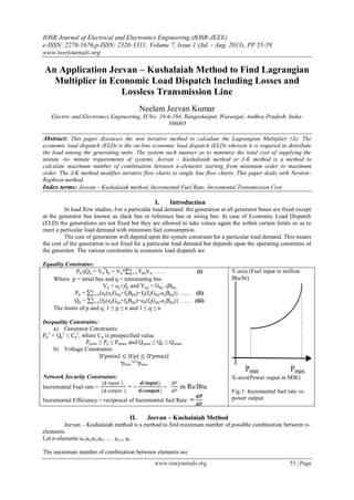
1. IOSR Journal of Electrical and Electronics Engineering (IOSR-JEEE)
e-ISSN: 2278-1676,p-ISSN: 2320-3331, Volume 7, Issue 1 (Jul. - Aug. 2013), PP 55-59
www.iosrjournals.org
www.iosrjournals.org 55 | Page
An Application Jeevan – Kushalaiah Method to Find Lagrangian
Multiplier in Economic Load Dispatch Including Losses and
Lossless Transmission Line
Neelam Jeevan Kumar
Electric and Electronics Engineering, H.No: 19-6-194, Rangashaipet, Warangal, Andhra Pradesh, India-
506005
Abstract: This paper discusses the non iterative method to calculate the Lagrangian Multiplier ( 𝜆). The
economic load dispatch (ELD) is the on-line economic load dispatch (ELD) wherein it is required to distribute
the load among the generating units. The system such manner as to minimize the total cost of supplying the
minute -to- minute requirements of systems. Jeevan – Kushalaiah method or J-K method is a method to
calculate maximum number of combination between n-elements starting from minimum order to maximum
order. The J-K method modifies iterative flow charts to single line flow charts. This paper deals with Newton-
Raphson method.
Index terms: Jeevan – Kushalaiah method, Incremental Fuel Rate, Incremental Transmission Cost
I. Introduction
In load flow studies, For a particular load demand the generation at all generator buses are fixed except
at the generator bus known as slack bus or reference bus or swing bus. In case of Economic Load Dispatch
(ELD) the generations are not fixed but they are allowed to take values again the within certain limits so as to
meet a particular load demand with minimum fuel consumption.
The cost of generation will depend upon the system constraint for a particular load demand. This means
the cost of the generation is not fixed for a particular load demand but depends upon the operating constrains of
the generator. The various constraints in economic load dispatch are
Equality Constrains:
Pp-jQp = Vp
*
Ip = Vp* Yn
q=1 pqVq …… (i)
Where p = intial bus and q = terminating bus
Vp = ep+jfp and Ypq = Gpq -jBpq
Pp = {𝑛
𝑞=1 ep(eqGpq+fqBpq)+fp(fqGpq-eqBpq)} …… (ii)
Qp = {𝑛
𝑞=1 fp(eqGpq+fqBpq)+ep(fqGpq-eqBpq)} …… (iii)
The limits of p and q: 1 ≤ p ≤ n and 1 ≤ q ≤ n
Inequality Constrains:
a) Generator Constraints:
Pp
2
+ Qp
2
≤ Cp
2
, where Cp is prespecified value.
Ppmin ≤ Pp ≤ Ppmax and Qpmin ≤ Qp ≤ Qpmax
b) Voltage Constraints:
𝑉𝑝𝑚𝑖𝑛 ≤ 𝑉𝑝 ≤ 𝑉𝑝𝑚𝑎𝑥
ᵟpmin
≤
ᵟ≤
ᵟpmax
Network Security Constraints:
Incremental Fuel rate =
(∆ input )
(∆ output )
= =
𝒅(𝐢𝐧𝐩𝐮𝐭)
𝒅(𝐨𝐮𝐭𝐩𝐮𝐭)
=
𝑑𝐹
𝑑𝑃
in Rs/Btu
Incremental Efficiency = reciprocal of Incremental fuel Rate =
𝒅𝑷
𝒅𝑭
Y-axis (Fuel input in million
Btu/hr)
X-axis(Power ouput in MW)
Fig.1: Incremental fuel rate vs.
power output
II. Jeevan – Kushalaiah Method
Jeevan – Kushalaiah method is a method to find maximum number of possible combination between n-
elements.
Let n-elements a1,a2,a3,a4, … an-1, an
The maximum number of combination between elements are

2. An Application Jeevan – Kushalaiah Method To Find Lagrangian Multiplier In Economic Load
www.iosrjournals.org 56 | Page
{(1),( a1,a2,a3,a4, … an-1, an),( a1a2, a1a3, a1a4, … a1an-1, a1an.. a2a3, a2a4, … a2an-1, a2an…… a3a4, a3a5, …
a3an-1, a3an…………. an-1an),( a1a2a3, a1a2a4, … a1a2an-1, a1a2an………an-2an-1an),…..,(…..),…….,(a1a2a3…an-
1an)}
….. (iv)
= {(ϴ0),( ϴ1),( ϴ2),…….( ϴp-1),( ϴp)}
Here ϴ0 = 1, ϴ1 = +,-,*,/ of all elements
( ϴp) = Addition or Subtraction or Multiplication or Division or a square Matrix.
Example - 1:
( ϴp) = (a,b)
 Addition = a + b
 Subtraction = a - b
 Multiplication = a*b
 Division = a/b
 Square Matrix =
𝑎11 12
21 𝑏22
(a and b are diagonal positions only.)
Commonly Multiplication and Addition is performed
ϴp = (n - (p-1)) p - 1 …….. ( v )
total number of combinations of n-elements
= ϴ0 +ϴ1 + ϴ2
𝑝=2 p ………. (vi)
The value of p ≥ 2
where is summator like factorial operation instead of multiplication addition is performed.
Example-2: (5)2 =5 = 5 +4 +3 +2 +1 = 5+4+3+2+1+4+3+2+1+3+2+1+2+1+1 = 35
III. Calculation of λ of ELD without Losses
The Load demand = PD
The generation of nth
unit = Pn
Total fuel input to the system = FT
The Fuel input tot nth
system = Fn
The system with without losses,PL = 0
PD = Pn
k=1 k ……… (vii)
The auxiliary function
F = FT+λ(PD - Pn
k=1 k)
Where λ is Lagrangian multiplier
Differentiating F with respect to Pn and equating to zero
𝐝𝐅𝟏
𝐝𝐏𝟏
=
𝐝𝐅𝟐
𝐝𝐏𝟐
=
𝐝𝐅𝐧
𝐝𝐏𝐧
= λ
Where
dFn
dPn
= incremental production cost of nth plant in
Rs. /MWhr
For a plant over a limited range Fig .2: Generalized diagram of a power
system without losses.
𝐝𝐅𝐧
𝐝𝐏𝐧
= FnnPn +fn = λ ……… (viii)
Where Fnn = slope of total incremental production curve and
fn = intercept of incremental production cost curve.
From equation number (viii), we have
Pn = (λassum – fn) / Fnn
P1 = (λassum – f1) / F11 , F2 = (λassum – f2) / F22………
Pn-1 = (λassum – fn-1) / Fn-1n-1 ,Pn = (λassum – fn) / Fnn
Total power to be generated PT is
PD = P1 + P2 +…..+ Pn

3. An Application Jeevan – Kushalaiah Method To Find Lagrangian Multiplier In Economic Load
www.iosrjournals.org 57 | Page
PD = {(λassum – f1) / F11 }+{(λassum – f2) / F22 }+…+{(λassum – fn) / Fnn } ………… (ix)
Rewriting equation-(ix) for direct calculation of λ
λassum = {PD ( 𝐅𝐧
𝐣=𝟏 jj) + 𝐟𝐧
𝐤=𝟏 k(ϕn-k-1)}/( 𝛟𝐧
𝐧=𝟏 𝐧) … … (x)
Where ϕn = elements combination in ϴn-1
IV. Calculation of λ of ELD without Losses
The system with without losses,PL
PD + PL = 𝐏𝐧
𝐤=𝟏 k ……… (xi)
The auxiliary function
F = FT + λ ( PD + PL - 𝐏𝐧
𝐤=𝟏 k )
𝐝𝐅𝐧
𝐝𝐏𝐧
+ 𝛌(
𝛛𝐏𝐋
𝛛𝐏𝐧
) = 𝛌 ….. (xii)
𝜕𝑃L
𝜕𝑃𝑛
= The Incremental Transmission Loss at plant – n
Loss formula approximately
PL = 𝐏𝐣 j 𝐏𝐤 k Bjk
Assumptions
 The equivalent load current at any bus remains constant.
 The generator bus voltage magnitude and angles are
constant.
 Power factor is constant
𝛛𝐏𝐋
𝛛𝐏𝐧
= 2 𝑷𝒋 jBjk ….. (xiii)
𝒅𝑭𝒏
𝒅𝑷𝒏
= FnnPn + fn ….. (xiv)
Fig . 3: Generalized diagram of a power
system with losses.
Substituting equations (xiii)(xiv) in (xii) we get
FnnPn+fn+2λ 𝐁mnPm = λ …… (xv)
Rewriting the equation - (xii)
𝐝𝐅𝐧
𝐝𝐏𝐧
+ 𝛌(
𝛛𝐏𝐋
𝛛𝐏𝐧
) = 𝛌 ,
𝛛𝐏𝐋
𝛛𝐏𝐧
= Ln
𝐝𝐅𝐧
𝐝𝐏𝐧
+ λLn = λ
𝐝𝐅𝐧
𝐝𝐏𝐧
= λ (1- Ln) …… (xvi)
From equation – (xiv) in (xvi)
FnnPn + fn = λ (1- Ln)
(FnnPn + fn)/( 1- Ln) = λ
Generation of n-generator Pn = {λ (1- Ln) – fn}/Fnn
P1 = {λ (1- L1) – f1}/F11 , P2 = {λ (1- L2) – f2}/F22 ………… Pn = {λ (1- Ln) – fn}/Fnn
PT = P1 +P2 + Pn = {λ (1- L1) – f1}/F11 + {λ (1- L2) – f2}/F22 +………… + {λ (1- Ln) – fn}/Fnn
Rewriting the above equation
λassum = {PD ( 𝐅𝐧
𝐣=𝟏 jj) + 𝐟𝐧
𝐤=𝟏 k(ϕn-k-1)} /( 𝛟𝐧
𝐧=𝟏 𝐧)(1-Ln) …….. ( xvii )
V. Algorithms and Flow Charts
V.a. Algorithm for ELD without Losses and ELD with losses
Step-I. Start and Read The Fuel input tot nth
system ( Fn ), Fnn = slope of total incremental production, The
Load demand ( PD )
Step-II. Calculate loss. For ELD without losses PL = 0
Step-III. Calculate λassum, and set bus number, n = 1, calculate Pn check all buses are completed or not, if yes
go to next step, if not increment n = n+1 repeat step-III
Step-IV Print Generation and calculate cost of generation.
Note: Algorithm for ELD without Losses and ELD with losses changes according to their transmission
line losses and operating conditions. In these algorithms are only for normal operation and not affected
for atmospheric changes like raining and snow falling on the line.

4. An Application Jeevan – Kushalaiah Method To Find Lagrangian Multiplier In Economic Load
www.iosrjournals.org 58 | Page
Flow chart for ELD without losses Flow chart for ELD with losses

5. An Application Jeevan – Kushalaiah Method To Find Lagrangian Multiplier In Economic Load
www.iosrjournals.org 59 | Page
V. Conclusion
In this method, the Calculated values are within the
limits of voltage constraints and generator i.e.,
𝑉𝑝𝑚𝑖𝑛 ≤ 𝑉𝑝 ≤ 𝑉𝑝𝑚𝑎𝑥 and
Ppmin ≤ Pp ≤ Ppmax and Qpmin ≤ Qp ≤ Qpmax
And there is iteration process to calculate Lagrangian multiplier λ,in the flow chart backward path is only for
calculating required output at generating stations not to finding out the λ. This method applied for Thermal and
Hydro power stations or connection of Hydro-Thermal Power station and Grid connections.
References
[1]. Neelam Jeevan Kumar,” Jeevan kushalaiah method to find the coefficients of characteristic equation of a
matrix and introduction of summetor”, 2229-5518, Volume 4, Issue 8,2013
[2]. I.A . Farhat , M.E. El-Hawar y, “Optimization methods applie d for solving the short-term hydrothermal
coordination problem”, 79 (20 09) 1308–1320, doi:10.1016/j.epsr.20 09.0 4.0 01
[3]. Y.H. Song, Modern Optimization Techniques in Power Systems, Kluwer Aca-demic Publishers,
Dordrecht, The Netherlands, 1999
[4]. J.A . Momoh, Electric Power System Applications of Optimization, Marcel Dekker, New York , 20 01.
[5]. Basic issues in Lagrangian optimization, in Optimization in Planning and Operation of Electric Power
Systems (K. Frauendorfer, H. Glavitsch and R. Bacher, eds.), Physica-Verlag, Heidelberg, 1993, 3-30 (by
R. T. Rockafellar)
[6]. R. T. Rockafellar “Lagrange Multipliers and Optimality”, 35(2), 183–238. (56 pages),
http://dx.doi.org/10.1137/1035044
[7]. book: C.L Wadhwa, ”Electrical power systems”, ISBN 978-81-224-2839-1
Author
The author is academic researcher, Department Electrical and Electronics Engineering. His
research areas are Optimization of Power system and applied mathematics.