1. Solution
Week 75 (2/16/04)
Hanging chain
We’ll present four solutions. The first one involves balancing forces. The other three
involve various variations on a variational argument.
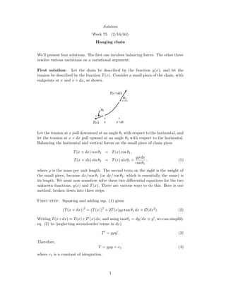
First solution: Let the chain be described by the function y(x), and let the
tension be described by the function T(x). Consider a small piece of the chain, with
endpoints at x and x + dx, as shown.
θ
θ
1
2
x+dxxT(x)
T(x+dx)
Let the tension at x pull downward at an angle θ1 with respect to the horizontal, and
let the tension at x + dx pull upward at an angle θ2 with respect to the horizontal.
Balancing the horizontal and vertical forces on the small piece of chain gives
T(x + dx) cos θ2 = T(x) cos θ1,
T(x + dx) sin θ2 = T(x) sin θ1 +
gρ dx
cos θ1
, (1)
where ρ is the mass per unit length. The second term on the right is the weight of
the small piece, because dx/ cos θ1 (or dx/ cos θ2, which is essentially the same) is
its length. We must now somehow solve these two differential equations for the two
unknown functions, y(x) and T(x). There are various ways to do this. Here is one
method, broken down into three steps.
First step: Squaring and adding eqs. (1) gives
(T(x + dx))2
= (T(x))2
+ 2T(x)gρ tan θ1 dx + O(dx2
). (2)
Writing T(x+dx) ≈ T(x)+T (x) dx, and using tan θ1 = dy/dx ≡ y , we can simplify
eq. (2) to (neglecting second-order terms in dx)
T = gρy . (3)
Therefore,
T = gρy + c1, (4)
where c1 is a constant of integration.
1

2. Second step: Let’s see what we can extract from the first equation in eqs. (1).
Using
cos θ1 =
1
1 + (y (x))2
, and cos θ2 =
1
1 + (y (x + dx))2
, (5)
and expanding things to first order in dx, the first of eqs. (1) becomes
T + T dx
1 + (y + y dx)2
=
T
1 + y 2
. (6)
All of the functions here are evaluated at x, which we won’t bother writing. Ex-
panding the first square root gives (to first order in dx)
T + T dx
1 + y 2
1 −
y y dx
1 + y 2
=
T
1 + y 2
. (7)
To first order in dx this yields
T
T
=
y y
1 + y 2
. (8)
Integrating both sides gives
ln T + c2 =
1
2
ln(1 + y 2
), (9)
where c2 is a constant of integration. Exponentiating then gives
c2
3T2
= 1 + y 2
, (10)
where c3 ≡ ec2 .
Third step: We will now combine eq. (10) with eq. (4) to solve for y(x). Elim-
inating T gives c2
3(gρy + c1)2 = 1 + y 2. We can rewrite this is the somewhat nicer
form,
1 + y 2
= α2
(y + h)2
, (11)
where α ≡ c3gρ, and h = c1/gρ. At this point we can cleverly guess (motivated by
the fact that 1 + sinh2
z = cosh2
z) that the solution for y is given by
y(x) + h =
1
α
cosh α(x + a). (12)
Or, we can separate variables to obtain
dx =
dy
α2(y + h)2 − 1
, (13)
and then use the fact that the integral of 1/
√
z2 − 1 is cosh−1
z, to obtain the same
result.
The shape of the chain is therefore a hyperbolic cosine function. The constant h
isn’t too important, because it simply depends on where we pick the y = 0 height.
Furthermore, we can eliminate the need for the constant a if we pick x = 0 to be
2

3. where the lowest point of the chain is (or where it would be, in the case where the
slope is always nonzero). In this case, using eq. (12), we see that y (0) = 0 implies
a = 0, as desired. We then have (ignoring the constant h) the nice simple result,
y(x) =
1
α
cosh(αx). (14)
We’ll show how to determine α at the end of the solutions.
Second solution: We can also solve this problem by using a variational argument.
The chain will want to minimize its potential energy, so we want to find the function
y(x) that minimizes the integral,
U = (dm)gy = ρ 1 + y 2 dx gy = ρg y 1 + y 2 dx, (15)
subject to the constraint that the length of the chain is some given length . That
is,
= 1 + y 2 dx. (16)
Without this constraint, we could find y(x) by simply using the Euler-Lagrange
equation on the “Lagrangian” y 1 + y 2 given in eq. (15). But with the constraint,
we must use the method of Lagrange multipliers. This works for functionals in the
same way it works for functions. Basically, for any small variation in y(x) near the
minimum, we want the change in U to be proportional to the change in .1 This
means that there exists a linear combination of U and that doesn’t change, to first
order in any small variation in y(x). In other words, the Lagrangian2
L = y 1 + y 2 + h 1 + y 2 = (y + h) 1 + y 2 (17)
satisfis the Euler-Lagrange equation, for some value of h. Therefore,
d
dx
∂L
∂y
=
∂L
∂y
=⇒
d
dx
(y + h)y
1 + y 2
= 1 + y 2. (18)
We must now perform some straightforward (although tedious) differentiations. Us-
ing the product rule on the left-hand side, and making copious use of the chain rule,
we obtain
y 2
1 + y 2
+
(y + h)y
1 + y 2
−
(y + h)y 2y
(1 + y 2)3/2
= 1 + y 2. (19)
Multiplying through by (1 + y 2)3/2 and simplifying gives
(y + h)y = (1 + y 2
). (20)
1
The reason for this is the following. Assume that we have found the desired function y(x)
that minimizes U, and consider two different variations in y(x) that give the same change in ,
but different changes in U. Then the difference in these variations will produce no change in ,
while yielding a nonzero first-order change in U. This contradicts the fact that our y(x) yielded an
extremum of U.
2
We’ll use “h” for the Lagrange multiplier, to make the notation consistent with that in the first
solution.
3

4. Having produced the Euler-Lagrange differential equation, we must now integrate
it. If we multiply through by y and rearrange, we obtain
y y
1 + y 2
=
y
y + h
. (21)
Taking the dx integral of both sides gives (1/2) ln(1 + y 2) = ln(y + h) + c4, where
c4 is a constant of integration. Exponentiation then gives (with α ≡ ec4 )
1 + y 2
= α2
(y + h)2
. (22)
in agreement with eq. (11).
Third solution: Let’s use a variational argument again, but now with y as the
independent variable. That is, let the chain be described by the function x(y). Then
the potential energy is
U = (dm)gy = ρ 1 + x 2 dy gy = ρg y 1 + x 2 dy. (23)
The constraint is
= 1 + x 2 dy. (24)
Using the method of Lagrange multipliers as in the second solution above, the
Lagrangian we want to consider is
L = y 1 + x 2 + h 1 + x 2 = (y + h) 1 + x 2. (25)
Our Euler-Lagrange equation is then
d
dy
∂L
∂x
=
∂L
∂x
=⇒
d
dy
(y + h)x
√
1 + x 2
= 0. (26)
The zero on the right-hand side makes things nice and easy, because it means that
the quantity in parentheses is a constant. Calling this constant 1/α (to end up with
the notation in the second solution), we have α(y + h)x =
√
1 + x 2. Therefore,
x =
1
α2(y + h)2 − 1
, (27)
which is equivalent to eq. (13).
Fourth solution: Note that our “Lagrangian” in the second solution above, which
is given in eq. (17) as
L = (y + h) 1 + y 2, (28)
is independent of x. Therefore, in analogy with conservation of energy (which arises
from a Lagrangian that is independent of t), the quantity
E ≡ y
∂L
∂y
− L = −
y + h
1 + y 2
(29)
4

5. is independent of x. Call it 1/α. Then we have reproduced eq. (11).
Remark: The constant α can be determined from the locations of the endpoints and
the length of the chain. The position of the chain may be described by giving (1) the
horizontal distance, d, between the two endpoints, (2) the vertical distance, λ, between the
two endpoints, and (3) the length, , of the chain, as shown.
d
λ
l
d-x-x x=00 0
Note that it is not obvious what the horizontal distances between the ends and the minimum
point (which we have chosen as the x = 0 point) are. If λ = 0, then these distances are
simply d/2. But otherwise, they are not so clear.
If we let the left endpoint be located at x = −x0, then the right endpoint is located at
x = d − x0. We now have two unknowns, x0 and α. Our two conditions are3
y(d − x0) − y(−x0) = λ, (30)
along with the condition that the length equals , which takes the form (using eq. (14))
=
d−x0
−x0
1 + y 2 dx
=
1
α
sinh(αx)
d−x0
−x0
. (31)
Writing out eqs. (30) and (31) explicitly, using eq. (14), we have
cosh α(d − x0) − cosh(−αx0) = αλ, and
sinh α(d − x0) − sinh(−αx0) = α . (32)
If we take the difference of the squares of these two equations, and use the hyperbolic
identities cosh2
x − sinh2
x = 1 and cosh x cosh y − sinh x sinh y = cosh(x − y), we obtain
2 − 2 cosh(αd) = α2
(λ2
− 2
). (33)
We can now numerically solve this equation for α. Using a “half-angle” formula, you can
show that eq. (33) may also be written as
2 sinh(αd/2) = α 2 − λ2. (34)
We can check some limits here. If λ = 0 and = d (that is, the chain forms a horizontal
straight line), then eq. (34) becomes 2 sinh(αd/2) = αd. The solution to this is α = 0,
which does indeed correspond to a horizontal straight line, because for small α, eq. (14)
behaves like αx2
/2 (up to an additive constant), which varies slowly with x for small α.
Another limit is where is much larger than both d and λ. In this case, eq. (34) becomes
2 sinh(αd/2) ≈ α . The solution to this is a very large α, which corresponds to a “droopy”
chain, because eq. (14) varies rapidly with x for large α.
3
We’ll take the right end to be higher than the left end, without loss of generality.
5