Build Your Own 3D Scanner: 3D Scanning with Structured Lighting
•
13 recomendaciones•23,156 vistas

Build Your Own 3D Scanner: 3D Scanning with Structured Lighting http://mesh.brown.edu/byo3d/ SIGGRAPH 2009 Courses Douglas Lanman and Gabriel Taubin This course provides a beginner with the necessary mathematics, software, and practical details to leverage projector-camera systems in their own 3D scanning projects. An example-driven approach is used throughout; each new concept is illustrated using a practical scanner implemented with off-the-shelf parts. The course concludes by detailing how these new approaches are used in rapid prototyping, entertainment, cultural heritage, and web-based applications.
![[object Object],[object Object],[object Object],[object Object],[object Object],[object Object],[object Object],Course Schedule](data:image/gif;base64,R0lGODlhAQABAIAAAAAAAP///yH5BAEAAAAALAAAAAABAAEAAAIBRAA7)
Recomendados
Más contenido relacionado
La actualidad más candente
La actualidad más candente (20)
Destacado
Destacado (20)
Similar a Build Your Own 3D Scanner: 3D Scanning with Structured Lighting
Similar a Build Your Own 3D Scanner: 3D Scanning with Structured Lighting (20)
Último
Último (20)
Build Your Own 3D Scanner: 3D Scanning with Structured Lighting
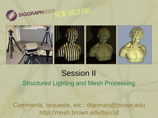
- 1. Session II Structured Lighting and Mesh Processing http://mesh.brown.edu/byo3d Comments, requests, etc.: dlanman@brown.edu
- 7. Additional Structured Lighting Patterns J. Salvi, J. Pag è s, and J. Batlle. Pattern Codification Strategies in Structured Light Systems . Pattern Recognition , 2004 “ Single-shot” patterns (N-arrays, grids, random, etc.) De Bruijn sequences [Zhang et al. 2002] Phase-shifting [Zhang et al. 2004] Spatial encoding strategies [Chen et al. 2007] Pseudorandom and M-arrays [Griffin 1992]
- 13. Demo: Camera Calibration in OpenCV 1 1 1 1 1 1 2 2 2 2 2 2 3 3 3 3 4 4 4 5 5 6 6 7
- 16. Demo: Projector Calibration in OpenCV 0.5 0.5 0.5 0.5 1 1 1 1 1.5 1.5 1.5 1.5 2 2 2 2 2.5 2.5 2.5 3 3 3 3 3.5 3.5 4 4 4.5 4.5
- 17. Structured Lighting Reconstruction Results
- 19. Demo: Putting it All Together
- 20. How to Get the Source Code http://mesh.brown.edu/byo3d
- 21. For More Details http://mesh.brown.edu/byo3d
Notas del editor
- Welcome back. In the first session we saw how to build low-cost 3D scanners using manually swept light/shadow planes. This has several drawbacks. First, to calibrate the illumination planes, we required a pair of planar patterns to be present within the scene. Second, the scanning process was slow and required manual interaction with the light source. We can eliminate these problems by using a digital projector to create the swept-planes. Furthermore, if we're clever, we can project carefully-selected patterns to allow the ray-plane correspondence to be rapidly assigned in a relatively small number of frames. Such patterns are known as “structured lighting”. In this first half of this session we analyze several structured lighting methods. In addition, we will describe the software and theory behind projector calibration. The second half of this session will describe how to extract a high quality mesh, suitable for interactive applications, from the noisy point cloud data produced by any of these scanners. In addition, we will briefly outline well-established methods for mesh processing, allowing gap-filling and smoothing to be applied to the acquired models.
- In this section we cover structured lighting.
- A simple projector-camera system is shown above, containing a pair of Point Grey Flea2 digital cameras and a single Mitsubishi XD300U projector. In the following discussion we'll assume that only one camera is being used. The primary benefit of introducing the projector is to eliminate the mechanical motion required in the previous systems. Assuming minimal lens distortion, we could simply use the projector to display one row or column at a time, as shown on the top right; thus, 768 or 1024 images would be required to assign the correspondences between camera pixels and projector rows or columns, respectively. If we again included a pair of calibration planes within the scene, then an identical swept-plane reconstruction pipeline could be applied. Such a strategy doesn't fully exploit the projector. Since we are now free to project arbitrary (possibly 24-bit) color images, there should be a sequence of coded patterns, besides simple translations of linear stripes, which allow the camera-projector correspondences to be assigned in relatively few frames. This is the central goal of structured lighting. If we assume reconstruction will be performed by ray-plane triangulation, then an image sequence is required that assigns a unique code to each projected plane. In general, the identity of each plane can be encoded spatially (i.e., within a single frame) or temporally (i.e., across multiple frames), or with a combination of both spatial and temporal encodings. There are benefits and drawbacks to each strategy. For instance, purely spatial encodings can allow a single static pattern to be used for reconstruction, allowing dynamic scenes to be captured. Alternatively, purely temporal encodings are more likely to benefit from redundancy, reducing reconstruction artifacts. A comprehensive assessment of such codes was presented by Salvi et al. [2003] (which is included in the course notes). For this course, we will focus on purely temporal encodings. While such patterns are not well-suited to scanning dynamic scenes, they have the benefit of being easy to decode and are very robust to surface texture variation, producing accurate reconstructions for static objects (with the normal prohibition of transparent or other problematic materials). As shown on the top-right, we could assign a unique color (or intensity) to each projector row or column. Such a pattern would be highly-sensitive to surface texture, and produces many artifacts in practice. A “classic” alternative to such spatial “ramp” patterns is to project a temporal sequence consisting of the individual bit-planes of the binary encoding of the integer projector row or column indices.
- A binary encoding of the projector rows (or columns) would require log 2 (x) frames, where x is the number of projector rows (or columns). Thus, a sequence of at least 10 frames must be projected to encode the projector rows (or columns). Such a sequence is shown in the top right, where each row represents a single bit-plane of the binary encoding of the projector columns. Note that this sequence is ordered such that the most significant bit is first. To clarify, an individual pixel in the projector is assigned a binary sequence, over at least 10 frames in this example; if we want to encode only the projector columns with this binary sequence, then a column in the sequence at the top right corresponds to the intensity of the corresponding column of pixels projected in each frame. In practice, such a sequence is easy to decode so long as the projector and camera(s) are synchronized. In practice, 2*log 2 (x) frames are projected – corresponding to the original binary sequence and its inverse. Thus, we can compare (on a per camera pixel basis) a given projected bit-plane and its inverse and determine whether a given camera pixel is brighter in the first or second image. If the original sequence is brighter at a given camera pixel, then the decoded bit is set high, otherwise the decoded bit is set low. Afterwards, the binary sequence decoded for each camera pixel can be converted back to an integer index. This index directly provides the correspondence between the given camera pixel and a projector row (or column).
- The binary structured light sequence was proposed by Posdamer and Altschuler [1981]. Shortly afterward, Inokuchi et al. [1984] proposed Gray codes as an alternative. Considering the projector-camera arrangement as a communication system, then a key question immediately arises; what binary sequence is most robust to the known properties of the channel noise process? At a basic level, we are concerned with assigning an accurate projector row/column to camera pixel correspondence, otherwise triangulation artifacts will lead to large reconstruction errors. The reflected binary code was introduced by Frank Gray in 1947. As shown in the top-right, the Gray code can be obtained by reflecting, in a specific manner, the individual bit-planes of the binary code. The key property of the Gray code is that two neighboring code words (i.e., neighboring columns in the figure at the top-right) only differ by one bit. Adjacent codes have a Hamming distance of unity. As a result, the Gray code structured light sequence tends to be more robust to decoding errors. Notice that both Gray codes and binary sequences require the same number of images, yet Gray codes tend to result in fewer reconstruction artifacts. The specific algorithm for converting a binary to Gray encoding is shown in the “Bin2Gray” pseudocode on the bottom right.
- The animated sequence on the top left shows the Gray code structured light sequence, as it illuminates a sculpture. The decoding algorithm, to obtain projector row/column and camera pixel correspondences, is straightforward. As previously described, we determine whether a bit is high or low depending on whether a projected bit-plane or its inverse is brighter at a given pixel. The temporal bit sequence, per camera pixel, is then converted from a Gray code to a binary code. The binary encoding is then converted to an integer index. Typical decoding results are shown here; in the middle figure, the projector row and camera pixel correspondence is represented with the typical “jet” color map (used in MATLAB). As you can see, the correspondences are resolved on a per-pixel basis and possess, at least visually, very few artifacts or outliers. Similar decoding results for projector columns are shown on the right. Note that, in order to resolve the projector row and column correspondence, for each camera pixel, a total of 42 images were projected. Two images, corresponding to “all on” and “all off” projected images, were used to measure the dynamic range per-pixel, as well as the surface texture. Twenty images were used to encode the projector rows, as well as 20 more to encode the projector columns.
- Image sources: http://grail.cs.washington.edu/projects/moscan/ Fast three-step phase-shifting algorithm (Peisen S. Huang and Song Zhang) http://ieeexplore.ieee.org/stamp/stamp.jsp?tp=&arnumber=4209129http://ieeexplore.ieee.org/stamp/stamp.jsp?tp=&arnumber=4209129 (Griffin et al.)
- Image sources: http://images.projectorpoint.co.uk/imagelibrary/projectors/InFocus/IN10/InFocus_LP70+large.jpg http://www.revolutionpc.net/xcart/images/T/Logitech-pro9000-L23-7280%20%20%20%201.jpg
- Image sources: http://opencv.jp/sample/camera_calibration.html
- We now turn to the topic of calibrating a projector in order to reconstruct a 3D point cloud from a structured light illumination sequence.
- In this course we use a popular method of projector calibration in which projectors are modeled as inverse cameras . In the first session, an ideal camera was modeled as a pinhole imaging system, with real-world cameras containing additional lenses. A camera was considered as a device that measures the irradiance along incident optical rays. The inverse mapping, from pixels to optical rays, required calibrating the intrinsic and extrinsic parameters of the camera, as well as a lens distortion model (the details of which are reviewed in the table shown here). A projector can be seen as the inverse of a camera, in which irradiances are projected, rather than measured, along optical rays. As for a camera, a given projector pixel can be mapped to a certain optical ray (practically a narrow cone of rays). Once again, an ideal projector can be modeled as a pinhole imaging system, with real-world projectors containing additional lenses that introduce distortion. A similar intrinsic model, with a principal point, skew coefficients, scale factors, and focal lengths can be similarly applied to projectors. As a result, we follow a similar calibration pipeline as used for our cameras.
- In order to calibrate a projector, we assume that the user has a camera which has been calibrated using the method from the first session. All that is required to calibrate the projector is a diffuse plain pattern with a small number of printed fiducials located on its surface; in our design, we used a piece of poster board with four printed checkerboard corners. A single image of the printed fiducials can be used, with the previous extrinsic camera calibration method, to recover the implicit equation of the calibration plane in the camera coordinate system. A projected checkerboard pattern is then displayed using the projector. Detected corners for the projected checkerboard are shown with green circles here. The corresponding pixels can be converted to rays using the inverse mapping for the camera. Afterwards, ray-plane intersection is used to recover a 3D position, in the world coordinate system, for each projected checkerboard corner. Now we recognize the key similarity with camera calibration. In the first session we showed how a set of correspondences, between 2D image coordinates and 3D points on the checkerboard pattern, could be used for estimating the parameters of the imaging model. A similar approach can now be applied for projector calibration. Once again, the Camera Calibration Toolbox for MATLAB can be used to recover the intrinsic and extrinsic projector calibration using the 2D-to-3D correspondences. Examples and source code will be discussed in the following live demonstration.
- To summarize, projector calibration naturally follows from camera calibration, when we consider projectors are inverse cameras . The MATLAB and C/C++ software included with the course materials will allow you the calibrate your projectors using the method outlined in this section. Typical calibration results for our design are shown on the right, with the viewing frusta for the cameras shown in red and the viewing frustum from the projector shown in green. Note that a single printed checkerboard, used for camera calibration, is shown by the red grid, whereas the recovered projected checkerboard is shown in green. Also note that the recovered camera and projector frusta correspond to the physical configuration shown on the left.
- To conclude this section, we return to the topic of structured light scanning. In the previous section we described how binary and Gray codes can be used to establish projector row/column correspondences for each camera pixel. To reconstruct a 3D point cloud, the implicit equation of each projected plane must be obtained. The previous calibration procedure can be used to establish the projected planes using the center of projection, as well as the inverse mapping from projector pixels to optical rays. The details of this implementation will be explained in the following live demonstration. Typical reconstruction results are shown in the animation on the right. As in the first session, the point cloud is rendered using a single color for each 3D point splat. Note that the reconstructed model is relatively free of outliers, except near points of tangency, where the optical ray from the camera is tangent to the object surface. In the following section we’ll describe methods to merge such point clouds, captured from multiple viewpoints, to form a complete representation of the object surface.