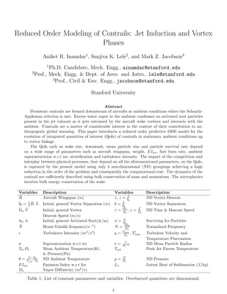
1. Reduced Order Modeling of Contrails: Jet Induction and Vortex
Phases
Aniket R. Inamdar1
, Sanjiva K. Lele2
, and Mark Z. Jacobson3
1
Ph.D. Candidate, Mech. Engg., ainamdar@stanford.edu
2
Prof., Mech. Engg. & Dept. of Aero. and Astro., lele@stanford.edu
3
Prof., Civil & Env. Engg., jacobson@stanford.edu
Stanford University
Abstract
Persistent contrails are formed downstream of aircrafts at ambient conditions where the Schmidt-
Appleman criterion is met. Excess water vapor in the ambient condenses on activated soot particles
present in the jet exhaust as it gets entrained by the aircraft wake vortices and interacts with the
ambient. Contrails are a matter of considerable interest in the context of their contribution to an-
thropogenic global warming. This paper introduces a reduced order predictive ODE model for the
evolution of integrated quantities of interest (QoIs) of contrails in stationary ambient conditions up
to vortex linkage.
The QoIs such as wake size, downwash, mean particle size and particle survival rate depend
on a wide range of parameters such as aircraft wingspan, weight, EIice, fuel burn rate, ambient
supersaturation w.r.t ice, stratification and turbulence intensity. The impact of the competition and
interplay between physical processes, that depend on all the aforementioned parameters, on the QoIs,
is captured by the present model using only 4 non-dimensional (ND) groupings achieving a huge
reduction in the order of the problem and consequently the computational cost. The dynamics of the
contrail are sufficiently described using bulk conservation of mass and momentum. The microphysics
involves bulk energy conservation of the wake.
Variables Description Variables Description
¯B Aircraft Wingspan (m) ¯z, z = ¯z
¯b0
ND Vortex Descent
¯b0 = π
4
¯B, ¯b Initial, general Vortex Separation (m) b =
¯b
¯b0
ND Vortex Separation
¯V0, ¯V Initial, general Vortex τ = t ¯V0
¯b0
, v =
¯V
¯V0
ND Time & Descent Speed
Descent Speed (m/s)
¯n0, ¯n Initial, general Activated Soot(#/m) n = ¯n
¯n0
Surviving Ice Particles
¯N Brunt-V¨ais¨al¨a frequancy(s−1) N =
¯N¯b0
¯V0
Normalized Frequency
Turbulence Intensity (m2/s3) q = vrms
¯V0
, Trms Turbulent Velocity and
Temperature Fluctuation
σ Supersaturation w.r.t ice r = ¯r
10−6 ND Mean Particle Radius
T0, P0 Mean Ambient Temperature(K) Tjet Peak Jet Excess Temperature
& Pressure(Pa)
θ = T−T0
Tjet−T0
ND Ambient Temperature p = P
P0
ND Pressure
EIice Emission Index w.r.t Ice Lv Latent Heat of Sublimation (J/kg)
Dv Vapor Diffusivity (m2/s)
Table 1: List of constant parameters and variables. Overbarred quantities are dimensional.
1

2. 1 Introduction
The IPCC report by Penner et. al. [18] that estimates the impact of aviation on the climate is
widely reported in literature. Lee et. al. [11] observed that the magnitude of climate impact in terms
of contribution to global anthropogenic radiative forcing for CO2 and Aviation Induced Cloudiness(AIC)
is comparable. While the influence of CO2 on climate change is relatively well understood, there is large
uncertainty in the influence of AIC on the climate. These uncertainties arise due to inadequate repre-
sentation (inaccurate parametrization) of contrails and contrail induced cirrus in GCMs that are used to
estimate these impacts. The CoCiP model by Schumann [20] uses some aircraft parameters, but the op-
tical properties are calculated coarsely, using an average effective size parameter for all contrail particles.
On the other hand, the GATOR model by Jacobson [9] does refined optical property calculations, but the
initialization of all contrails is identical for all aircrafts and ambient conditions.
It is the authors’ contention that it is necessary to better parametrize contrails to help reduce the
aforementioned uncertainties. Earlier attempts to model plume chemistry are reported in literature [16]
but there is need to develop effective parametrized models for contrails [17]. Given the large number and
wide range of parameters that affect contrails, it is computationally infeasible to span the entire parameter-
space with sufficient number of full scale simulations and generate “curve-fit” models for predicting contrail
QoIs with reasonable confidence. Thus, it becomes necessary to leverage the physical insight developed
from a limited number of simulations with carefully chosen parameters and develop a predictive model
that captures the most prominent physical processes. This paper presents one such parametrization of
contrails in the form of an ODE model on aircraft, ambient and microphysical parameters.
In Sec. 2 we provide a brief description of the LES model, cases and data that we use to infer qualitative
trends for the ODE model to capture. In Sec. 3 we outline the ODE model and provide justification for
the choices made therein followed by results and discussion of the model in Sec. 4. In sec. 5 we describe
our ongoing work followed by conclusions in sec. 6.
2 Large Eddy Simulations
2.1 LES Code and Case Parameters
We use a 3-D incompressible Navier − Stokes solver on unstructured grids to simulate the time-
evolution of a contrail in a stationary ambient from an age of 1sec. up to 1200sec. The ice particles are
tracked using Lagrangian particle tracking. Details of the fluids solver may be found in [13, 14]. The ice
particle growth is modeled using capacitive growth models described in [19, 8, 13, 6, 7]. In Table 2, we list
all LES cases performed and used in this study. Only one parameter is changed between any case and the
baseline, thus isolating the impact of said parameter. We choose the baseline ambient to be representative
of a cruise altitude of 10.5km [24].
Case Parameter Values
Baseline ¯B = 50m, ¯V0 = 1.5m/s, = 10−4m2/s3, vrms = 0.08m/s, ¯N = 0.01s−1,
σ = 1.3, EIice = 1015
Large Same as Baseline except ¯B = 70m
Small Same as Baseline except ¯B = 30m
Heavy Same as Baseline except ¯V0 = 2m/s
Light Same as Baseline except ¯V0 = 1m/s
EIice Same as Baseline except EIice = 1014 (from Naiman [13])
Stratification Same as Baseline except ¯N = 0.015s−1
Supersaturation w.r.t. Ice Same as Baseline except σ = 1.1 (from Naiman [13])
Table 2: List of LES cases
2

3. (a) Jet Phase(1s) (b) Induction Phase(15s)
(c) Vortex Phase(60s) (d) Dispersion Phase(600s)
Figure 1: Phases of Contrail Evolution
2.2 Inferences from LES data
In fig. 1, we have shown flight-direction averaged plots of contrail ice volume for the “Large” case. The
lifespan of a contrail may be split into 4 phases - jet, induction, vortex and dispersion. The jet phase is
when the warm jet exhaust, assumed to have a gaussian temperature distribution, is yet to be entrained
3

4. by the wake vortices. We assume all emitted soot particles are active for vapor deposition and that all the
emitted vapor has condensed uniformly on these active soot particles 1s behind the aircraft. So, the jet
phase is dependent solely on aircraft parameters. During this time, the trailing wing-tip vorticity rolls up
into 2 counter-rotating vortices whose strength (i.e. circulation Γ) depends on aircraft parameters.
Once the wake vortex pair is formed, it begins to induct the jet exhaust, marking the beginning of
the induction phase. The jet exhaust begins to cool as it interacts with the ambient air within the wake
oval. The counter-rotating pair of vortices induces downward motion on each other and this downward
motion is characteristic of the vortex phase. As the wake descends through the stably stratified ambient,
buoyancy retards the wake oval and simultaneously compresses it laterally, causing the vortices to come
closer to each other. Vortices are eventually consumed by catastrophic destruction of vorticity once the
vortex cores come sufficiently close to each other. This is followed by buoyant sloshing of the plume and
dispersion due to ambient turbulence.
It is pertinent to observe that the turbulent mixing time scale (vrms
2
) at the wake oval boundary is
much larger as compared to the wake descent time scale (
¯b0
¯V0
) , implying that till the end of the vortex
phase, the impact of turbulent mixing on the dynamics of the contrail wake is negligible as is observed
in fig. 5. The evolution of the wake oval under stable stratification shows that the wake gets compressed
symmetrically about the vertical (Z) axis (see fig. 2), i.e. the wake is compressed symmetrically along its
semi-major axis.
X
Z
Vortex 1
0.865 b
1.045 b
Vortex 2
Separating Streamline
V
Fvisc
Fturb
Fbuoy
V
Figure 2: A schematic of the wake oval
2.2.1 Induction Phase
The induction of the jet exhaust by the trailing vortices is shown in fig. 3 for the baseline. The quantity
plotted is T−T0
Tjet−T0
, i.e. the excess temperature over ambient normalized by peak jet excess temperature. For
the baseline case, the peak jet excess temperature is 5K. In fig. 4, the particle survival and size growth
as observed in the LES data is plotted for various cases. The cut-off between the induction and vortex
phases is clearly visible – the particles start growing only in the vortex phase and correspondingly, the
survival rate is 1 in the induction phase. Knowing that the jet exhaust is warmer than the ambient and
that the process of induction cools the exhaust, we contend that the ice particle growth will not commence
until the mean temperature of the exhaust gas being inducted by the vortices falls sufficiently and the time
at which growth begins will thus be proportional to the rate of induction of the exhaust.
4

5. (a) t = 1s (b) t = 10s (c) t = 20s
Figure 3: Potential Temperature in the Induction Phase
0 0.5 1 1.5 2 2.5 3
0.2
0.3
0.4
0.5
0.6
0.7
0.8
0.9
1
τ
n
Particle Survival (LES)
Baseline
Large
Small
Heavy
Light
Low RHi
0 0.5 1 1.5 2 2.5 3
0.5
0.6
0.7
0.8
0.9
1
1.1
1.2
1.3
1.4
1.5
τ
r
Particle Size (LES)
Baseline
Large
Small
Heavy
Light
Low RHi
(a) (b)
Figure 4: (a) Particle Survival (b) Particle Size up to Vortex Linkage
2.2.2 Vortex Phase
The descent of the wake oval through the stratified ambient is shown in fig. 5. The argument made
about turbulent mixing time scale and vortex descent time scale implies that the interior of the wake is
largely insulated from the cool ambient. The temperature within the wake oval, barring the vortex cores,
remains largely uniform till the end of the vortex phase, as observed in the LES data. We are now tasked
with identifying the cause for this particular behavior. We can find a temperature, say Twake, (greater than
the ambient temperature) where the saturation pressure Psat
wake is equal to the vapor pressure w.r.t. ice for
a given ambient temperature and supersaturation (i.e. Psat
(Twake) = σPsat
(T0)). As the temperature falls
below this value, the excess vapor deposits on available activated particles releasing latent heat of fusion
causing a corresponding rise in temperature of the wake. This interplay is discussed in greater detail in
sec. 4. Thus the descent of the wake through stably stratified ambient is “isothermal”.
5

6. (a) t = 35s (b) t = 50s (c) t = 65s
Figure 5: Potential Temperature in the Vortex Phase
We now proceed to formalize the ODE model.
3 Model Description
It is known that the Greene’s model [3] gives conservative estimates for the decay and downward motion
of aircraft wake vortices i.e. it over-predicts the downwash and the vortex destruction time [2, 5]. This
may be attributed to the fact that it assumes the vortex separation to remain constant. We know that
the baroclinic term in the vorticity equations results in a inward motion of the vortex pair in presence of
stable stratification (cf. fig. 9 in [4]) as vorticity accumulates above and outside the wake oval. While a
model for vortex decay in stable stratification is provided in [2], it is based on a “curve fit” approach that
limits its predictive capability as it operates in the low Re range ∼ O(103
). The discussion that follows,
we will consider equations of motion for a wake of unit length in flight direction and all comparisons with
LES will be on a flight-direction averaged basis.
3.1 Greene’s Model
Using the Greene’s model [3] for a wake vortex system, the wake oval comprising of the counter
rotating vortices and the air entrained by them may be approximated to be of an initial cross-sectional size
A0 = π
4
(1.73)(2.09)¯b2
0, where 2.09
2
¯b0, 1.73
2
¯b0 are the semi-major and semi-minor axes of the oval. Qualitatively,
this oval is pushed downwards due to the initial impulse (2πρ¯b2
0
¯V0) from the aircraft and is acted upon by
viscous and turbulent drag and buoyancy. These forces are given as (cf. eqns. 1,8 &11 in [3]) :
Fvisc = −
ρ¯V 2
2
CDL
Fturb = −
ρ¯V 2
2
(4.93
vrms
¯V
)L
Fbuoy = −ρA ¯N2
¯z
(3.1)
where CD is the coefficient of drag taken to be 0.2, L is the lateral dimension of the oval with initial
value L0 = 2.09¯b0 and vrms is the RMS turbulent fluctuation in fluid velocity. A = π
4
(1.73)(2.09)¯b0
¯b, where
b is the separation between the cores and z is the descent at a given time. The expression 4.93vrms
¯V
may
be considered as a variable coefficient of turbulent drag. We draw attention to the fact that the numerical
values, {2.09, 1.73, 4.93}, are inherited from [3]. The dimensions of the initial wake oval {2.09¯b0, 1.73¯b0}
6

7. are the numerical values where the separating streamline is calculated to be, for a Lamb-Oseen vortex pair.
The value 4.93 is a “best guess” as described in [3] and is subject to uncertainty. Physically, turbulent
mixing at the wake oval and turbulent decay of the vortex cores causes the separating streamline to
recede and consequently, the downward velocity to reduce. Thus the Fturb factor may be interpreted as a
representation of this physical process.
3.2 Proposed ODE model
3.2.1 Dynamic Model
In keeping with the spirit of the Greene’s model, we consider our control volume (CV) to be the
variable-mass, variable-volume CV enclosed within the instantaneous mean separating streamline of the
wake system.
We propose to consider an inward force due to buoyancy acting on the foci of the wake oval to account
for the faster vortex decay and get better approximation to the vortex downwash and lifespan. To the
system in eqn. 3.1, we add a compressive force,
Fcomp = −1.73ρ ¯N2
¯z2¯b0 (3.2)
This term arises from considering the effect of pressure acting on the surface of the wake oval as follows:
Fcomp = ∆p
half-oval
dAoval ·ˆi and the integral is simply the vertical extent of the oval
∴ Fcomp = ∆p(1.73¯b0) = (∆ρg¯z)(1.73¯b0) = ((−ρ ¯N2
¯z)¯z)(1.73¯b0) = −1.73ρ ¯N2
¯z2¯b0
(3.3)
Noting that d¯z
d¯t
= ¯V , we get the following set of equations for the dynamics of the wake oval:
d(Downward Momentum of Wake)
dt
= Fvisc + Fturb + Fbuoy
⇒
d(2πρ¯b2 ¯V )
d¯t
= −
ρ¯V 2
2
CD(2.09¯b) −
ρ¯V 2
2
(4.93
vrms
¯V
)(2.09¯b) − ρ
π
4
(2.09¯b)(1.73¯b0) ¯N2
¯z
(3.4)
d(1
2
Masswake(inward velocity))
dt
= Fcomp
⇒
d(1
2
Aρd¯b
d¯t
)
d¯t
= −1.73ρ ¯N2
¯z2¯b0
(3.5)
Simplifying and introducing the corresponding non-dimensional(ND) quantities as in table 1, we get
the following governing equations:
ztt = −
1
b
2.09
1
20π
z2
t +
1.73
8
N2
z +
4.93
4π
qzt + 2btzt
btt = −
1
b
16N2
z2
2.09π
+ b2
t
(3.6)
These equations are limited by the vortex cores closely approaching each other followed by catastrophic
vortex core destruction. This is termed as the end of the vortex phase.
7

8. 3.2.2 Microphysical Model
In order to predict the normalized mean particle size r, we use the capacitive microphysical growth
models as described in [19, 8, 6, 13] averaged over the mean cross section of the contrail.
dmice
dt
= 4πDvΛ∆ρvapor = 4πDvΛρair(X − Xsat) (3.7)
Where Λ = C¯r is a measure of particle size, C being a correction factor to accommodate for asphericity
of ice particles, and X is the vapor mole fraction such that,
X =
Pvapor
P0
Xsat =
Psat
P0
X =
(1 + )Y
1 + Y
=
Mair
MH2O
− 1 (3.8)
The Psat is obtained using data from [12] as follows
Psat = K exp (9.550426 −
5723.265
T∗
wake
+ 3.53068 log (T∗
wake) − 0.00728332T∗
wake) (3.9)
Where T∗
wake = Twake − Trms
2
, and K = exp
2γMH2O
¯rRuT∗
wakeρice
is the Kelvin effect factor, γ being surface
tension and Ru, the universal gas constant. Simplifying eqn. 3.7 and introducing ND variables, we get the
following:
d¯r2
d¯t
=
2Dv
RuT0ρice
(σPsat(T0) − Psat(T∗
wake))
(r2
)t =
ρair
ρice
2Dv
¯b0
10−12 ¯V0Mair
(σp(T0) − p(T∗
wake))
(3.10)
This are exactly as eqn. 9 in [14], with the diffusion growth factor (G(Kn)) therein, assumed to be 1
as persistent contrails are observed in ambients cold enough for the microphysics to always be diffusion-
limited.
The particle survival is calculated using energy balance on our CV and enforcing the isothermal wake
condition discussed earlier. Thus, from the second law of thermodynamics, dU = dQ − dW, we have
dQwake = dWwake, i.e. latent heat of sublimation added to the wake is equal to the work done by the wake.
Taking rates on both sides,
d(Latent Heat)
dt
=
d(Work done to overcome visc. and turb. drag)
dt
+
d(Work done to overcome buoyancy)
dt
+
d(Work done against compression)
dt
∴
d(Lv
4
3
πρice¯r3
¯n)
dt
= −
d¯z
dt
(Fvisc + Fbouy + Fturb) − 2
d¯b
dt
Fcomp
If ¯n is the number of active particles at a given time, the evolution of ¯n is given by the following
equation:
d¯n
d¯t
= −
3
2
¯n
¯r2
d¯r2
d¯t
+
ρair
ρice
1
Lv ¯r3
3.62 ¯N2
¯z2¯b0
d¯b
d¯t
+ 0.75
d¯z
d¯t
1.33(
d¯z
d¯t
)2¯b + 0.9 ¯N2
¯z¯b¯b0 + 1.23vrms
¯b
d¯z
d¯t
(3.11)
Note that each term in the square bracket on the RHS of the above equation corresponds to work done
by terms on the RHS of eqns. 3.4, 3.5 and numerical coefficients have been simplified for conciseness.
Non-dimensionalizing results in:
8

9. dn
dt
= −
3
2
n
r2
dr2
dt
+
ρair
ρice
¯V 3
0
¯b0
10−18¯n0Lvr3
3.62N2
z2 db
dt
+ 0.75
dz
dt
1.33(
dz
dt
)2
b + 0.9N2
zb + 1.23qb
dz
dt
(3.12)
Note that the coefficient in front of the terms in the square bracket makes the dependence of survival
rate on EIice explicit, by virtue of the ¯n0 term in the denominator. The terms containing N2
include the
impact of stratification on survival rate, but this is not as significant as compared to the other terms in
the square bracket.
4 Results and Discussion
Following this, the equations for the dynamics of the wake oval up to the end of the vortex phase were
solved for various aircraft types and ambient conditions. Fig. 6 shows the normalized vortex separation
and descent. Key features of the dependence of contrail dynamics on aircraft and ambient parameters
as observed in literature [22, 21, 23] are captured by this simple ODE model. For higher stratification,
the initial downward impulse to the wake oval is the same as the baseline, but the Fcomp ∝ N2
(eqn.
3.2) is higher and consequently the vortex cores approach each other faster and the vortex lifespan and
descent is diminished. Higher turbulence as compared to the baseline causes the wake to have a diminished
descent Fturb ∝ vrms (eqn. 3.1), but a longer lifespan since the stratification, and consequently the rate of
approach of the vortex cores, is identical. For heavy (correspondingly light) aircrafts, the descent is higher
(correspondingly lower) compared to the baseline as the initial downward impulse on the wake is higher
(correspondingly lower) under identical stratification.
0 0.5 1 1.5 2 2.5 3 3.5 4 4.5
0
0.5
1
1.5
2
2.5
3
τ
NormalizedQuantities
Descent(solid) and Separation(dashed)
Baseline
Large
Small
Heavy
Light
High Strat.
High Turb.
Figure 6: Wake Vortex Dynamics
In fig. 7 the wake size and downwash as predicted by the ODE model is compared with the maximum
extent of ice particles for the baseline, heavy, large and higher stratification cases. Clearly, the assumption
of the contrail being entirely contained in the wake oval up to vortex linkage is a reasonable assumption.
The simple ODE model is able to predict, with reasonable accuracy, the dynamical behavior of the contrail
behind the aircraft. It is clear (see dotted contours in each case) that the model begins to deviate from
the behavior predicted by LES towards the very end of the vortex phase. This may be attributed to the
fact that the cores of the vortices are of finite size while the model assumes point vortices at the foci of the
oval. Thus, the process of catastrophic destruction of vorticity initiates earlier than the ODE prediction.
9

10. (a) Baseline (20s, 40s, 60s) (b) Heavy (20s, 35s, 50s)
(c) Large (20s, 40s, 60s) (d) High Strat. (20s, 35s, 50s)
Figure 7: Performance of the ODE model vs. LES data. Black patterned lines are furthest extent of LES
plumes and corresponding blue patterned lines are ODE wake ovals. Dot-dash: Late Induction, Solid: Mid
Vortex, Dotted: Late Vortex
In fig. 8(a,b), the model’s ability to capture the decay of particles during adiabatic compression and
mean particle size growth is clearly illustrated. Note that the initial induction phase where the particle size
doesn’t increase and no particles are lost due to evaporation as seen in the LES is adequately captured by
the ODE model using Twake as defined in sec. 2. For high EIice, the second term in eqn. 3.12 is negligible
and we observe that in order for the wake to maintain its temperature at Twake, the latent heat released
during growth of some particles, is used up to evaporate other particles, i.e. particle growth occurs at
the expense of survival rate of particles. Another interesting and promising observation is to be made
10

11. here. The evolution of particle size in the LES is governed by highly non-linear coupled equations. But,
the mean particle size growth is adequately and inexpensively tracked by the ODE model using the mean
thermodynamic properties of the wake oval!
0 0.5 1 1.5 2 2.5 3
0.2
0.3
0.4
0.5
0.6
0.7
0.8
0.9
1
τ
n
Particle Survival (LES)
0 0.5 1 1.5 2 2.5 3
0.2
0.3
0.4
0.5
0.6
0.7
0.8
0.9
1
τ
n
Particle Survival (LES)
Baseline
Large
Small
Heavy
Light
Low RHi
0 0.5 1 1.5 2 2.5 3
0.5
0.6
0.7
0.8
0.9
1
1.1
1.2
1.3
1.4
1.5
τ
r
Particle Size (LES)
0 0.5 1 1.5 2 2.5 3
0.2
0.3
0.4
0.5
0.6
0.7
0.8
0.9
1
τ
n
Particle Survival (LES)
Baseline
Large
Small
Heavy
Light
Low RHi
(a) (b)
Figure 8: (a) Particle Survival (b) Particle Size up to Vortex Phase. Solid lines are LES data and dashed
lines are the corresponding ODE model predictions
In fig. 9 (a,b) the impact of low EIice and high stratification is captured. When the EIice is low,
the corresponding ¯n0 is lower causing the second term in eqn. 3.12 to be non-trivial. Physically, we may
interpret this result as follows: Since the total number of ice particles is low, the latent heat released by
the growth of the surviving particles is not significant and the air in the wake is a large enough sink for this
heat to not affect the isothermal nature of the wake in any significant way. In case of higher stratification,
the turbulent fluctuations in temperature Trms are lower than in case of the baseline and this causes the
observed slower growth in mean particle size. Correspondingly, the survival rate is higher as compared to
the baseline.
0.5 1 1.5 2 2.5
0.5
0.6
0.7
0.8
0.9
1
1.1
τ
n
Particle Survival (LES)
Baseline LES
Baseline ODE
High Strat. LES
High Strat. ODE
Low EI LES
Low EI ODE
0.5 1 1.5 2 2.5
0.5
1
1.5
2
2.5
τ
r
Particle Size (LES)
Baseline LES
Baseline ODE
High Strat. LES
High Strat. ODE
Low EI LES
Low EI ODE
(a) (b)
Figure 9: (a) Particle Survival (b) Particle Size up to Vortex Phase. Solid lines are LES data and dashed
lines are the corresponding ODE model predictions
11

12. 5 Ongoing Work
5.1 Dispersion Phase
(a) Baseline 600s (b) Large 600s
Figure 10: Ice Volume in Primary and Secondary Plumes. The primary plume for the Large case is virtually
nonexistent.
Following the destruction of the wake vortices, the warm plume that has descended through stable
stratification is sloshed upwards. At the end of buoyant sloshing of the plume, a primary and secondary
plume of different sizes are formed, based on various parameters, as seen in our LES results (fig. 10) and
also in available literature, e.g. [23]. Beyond this, the spreading of the contrail is governed solely by the
ambient turbulence.
0.7 0.8 0.9 1 1.1 1.2 1.3
x 10
4
0.05
0.1
0.15
0.2
0.25
0.3
0.35
0.4
0.45
0.5
Time (s)
Velocity(m/s)
vx
vy
vz
Figure 11: Anisotropy of Ambient Turbulence under Stratification
12

13. Under stable stratification, turbulence becomes anisotropic as the fluctuations in the direction of strat-
ification are limited by the Ozmidov length scale [10, 1]. The spreading of the contrail in the directions
perpendicular to stratification is then governed by the characteristic velocity scale ¯vxz. In fig. 11, this
anisotropy under stratification is shown for the baseline case. Note that ¯
¯N
= 0.1m/s which is exactly
the value about which ¯vy oscillates.
TKE =
1
2
(¯v2
x + ¯v2
y + ¯v2
z ) | ¯vx = ¯vz = ¯vxz (homogeneous directions) (5.1)
¯vxz = TKE −
1
2
¯
¯N
| ¯v2
y ∼
¯
¯N
(Buoyancy Velocity Scale) (5.2)
In fig. 12, we have shown the evolution of ice mass in the dispersion phase. Since at present, the ODE
model is unable to model the buoyant sloshing, the ODE model was initialized using the total ice mass and
contrail dimensions using LES data at the end of the sloshing regime. The particle survival rate is held
constant at a value equal to that at the end of the vortex phase, as the ambient is now an infinite sink for
the latent heat of sublimation released by growing particles and work terms are non-existent as the vortex
oval doesn’t exist. The plume is simply allowed to spread laterally at a velocity of ¯vxz
2
and accrue ice mass
unabated at a uniform rate given in eqn. 3.10
400 500 600 700 800 900 1000 1100 1200
0
0.2
0.4
0.6
0.8
1
1.2
time(s)
icemass(kg/m)
LES vs. ODE in Dispersion Phase
High EI
Small
Large
Light
Heavy
Low RHi
Figure 12: Interim Results for Dispersion Phase
At present, the model is unable to accommodate the effects of turbulence and shear. For high values
of turbulent dissipation = O(10−3
)m2
/s3
, the turbulent mixing time is comparable to vortex downwash
time. This necessitates modification of the dynamical equations. Besides, the turbulent fluctuations in
temperature will also be higher, resulting in higher growth rate. The impact of realistic values of ambient
shear is to simply overpower that of stratification and should be included in the model.These will be
pursued to complete the model in terms of its predictive capability. The plume dilution model in [15]
captures the effect of shear effectively and our ODE model will be compared against it.
13

14. 6 Conclusions
In conclusion, we have demonstrated that the simple ODE model that captures the most prominent
physical processes governing the dynamics and microphysics of a contrail up to vortex linkage is indeed
able to predict integrated quantities of interest within reasonable confidence. As seen in fig. ??, with
just bulk momentum conservation, the model tracks both the lifespan and the downwash of the contrail
plume very closely. The largest error w.r.t LES data in downwash prediction, observed in the Large case,
was 15%. Complex non-linear processes governing ice particle growth can be reasonably modeled using
a simple concept of “Wake Oval Temperature” to predict mean particle size within a maximum of 10% of
LES data (largest error is in the Light case). As seen in figs. 8(a) and 9(a), particle survival rate under
various conditions is captured almost exactly using only bulk energy balance in this model. The ability of
this model to predict long-time dispersion also looks promising.
The model captures the dependence of the dynamics of the contrail on ambient and aircraft parameters
such as wingspan, weight, emission index w.r.t ice, stratification, relative humidity w.r.t ice, etc. Non-
dimensional coefficients arising naturally in the ODE model provide insight into the competition between
different processes driving the evolution of the contrail. In the table below, the 4 non-dimensional groups
are listed along with the physical properties they capture the impact of.
Nos. ND Grouping Name & Description
1 N =
¯N¯b0
¯V0
Normalized Frequency. Captures
Stratification, Weight and Size of Aircraft
2 q = vrms
¯V0
Normalized Turbulent Fluctuations. Captures
Turbulence Intensity and Aircraft Weight
Twake Mean Wake Temperature. Captures Fuel Burn Rate
T∗
wake = Twake − Trms
2
Mean Particle Temperature. Captures Turbulence
Intensity & Fuel Burn Rate
3 Growth Rate Factor. Captures
G = ρair
ρice
2Dv
¯b0
10−12 ¯V0Mair
(σp(T0) − p(T∗
wake)) Aircraft Weight, Size, Fuel Burn Rate,
Turbulence Intensity, RHi
4 S =
¯V 3
0
¯b0
10−18 ¯n0Lv
Survival Factor. Captures EIice, Aircraft Size and Weight
Table 3: Non-Dimensional Groupings
Acknowledgements
This project is sponsored by the Federal Aviation Administration under the award number DTFAWA-
05-D-0006. TeraGrid and XSEDE resources LONI, NCSA, KRAKEN and STAMPEDE under grant num-
ber TG-CTS080041N were used for this research. A.R.Inamdar would like to thank Dr. A.D.Naiman for
his invaluable help.
References
[1] D.Chung and G. Matheou. Direct numerical simulation of stationary homogeneous stratified sheared
turbulence. Journal of Fluid Mechanics, 696:434–467, 2012.
[2] J. F. Garten, J. Werner, D. C. Fritts, and S. Arendt. Direct numerical simulations of the Crow
instability and subsequent vortex reconnection in a stratified fluid. Journal of Fluid Mechanics,
426:1–45, 2001.
14

15. [3] G. C. Greene. An Approximate Model of Vortex Decay in the Atmosphere. Journal of Aircraft,
23(7):566–573, 1986.
[4] F. Holz¨apfel and T. Gerz. Two-dimensional wake vortex physics in the stably stratified atmmphere.
Aerosp. Sci. Technol., 5:261–270, 1999.
[5] F. Holz¨apfel, T. Gerz, and R. Baumann. The turbulent decay of trailing vortex pairs in stably stratified
environments. Aerosp. Sci. Technol., 5:95–108, 2001.
[6] A. R. Inamdar, S. K. Lele, and M. Z. Jacobson. A Probabilistic Ice Habit Model for LES of Contrails.
5th AIAA Atmospheric and Space Environments Conference, 2013.
[7] A. R. Inamdar, S. K. Lele, and M. Z. Jacobson. LES of Contrails With Ice Habit Treatment Using
the Fickian-Distribution Model. ASME 4th Joint US-European Fluids Engineering Division Summer
Meeting, 2014.
[8] M. Z. Jacobson. Fundamentals of Atmospheric Modeling. Cambridge University Press, Cambridge,
UK, 1999.
[9] M. Z. Jacobson. GATOR-GCMM A global- through urban-scale air pollution and weather forecast
model 1. Model design and treatment of subgrid soil, vegetation, roads, rooftops, water, sea ice, and
snow. Journal of Geophysical Research, 106(D6):5385–5401, 2001.
[10] Y. Kimura and J. R. Herring. Energy spectra of stably stratified turbulence. Journal of Fluid
Mechanics, 698:19–50, 2012.
[11] D. S. Lee, D. W. Fahey, P. M. Forster, P. J. Newton, R. C. N. Wit, L. L. Lim, B. Owen, and R. Sausen.
Aviation and global climate change in the 21st century. Atmospheric Environment, 43:3520–3537,
2009.
[12] D. M. Murphy and T. Koop. Review of the vapour pressures of ice and supercooled water for at-
mospheric applications. Quarterly Journal of the Royal Meteorological Society, 131(608):1539–1565,
April 2005.
[13] A. D. Naiman. Modeling Aircraft Contrails and Emission Plumes for Climate Impacts. PhD thesis,
Stanford University, 2011.
[14] A. D. Naiman, S. K. Lele, and M. Z. Jacobson. Large Eddy Simulations of Contrail Development:
Sensitivity to Initial and Ambient Conditions over First Twenty Minutes. Journal of Geophysical
Research, D21208, 2011.
[15] A. D. Naiman, S. K. Lele, J. T. Wilkerson, and M. Z. Jacobson. Parameterization of Subgrid Plume Di-
lution for use in Large-Scale Atmospheric Simulations. Atmospheric Chemistry and Physics, 10:2551–
2560, 2010.
[16] R. Paoli, D. Cariolle, and R. Sausen. Review of effective emissions modeling and computation. Geosci.
Model Dev., 4:643–667, 2011.
[17] Roberto Paoli and Karim Shariff. Contrail modeling and simulation. Annu. Rev. Fluid Mech., 48:393–
427, 2016.
[18] J. E. Penner, D. H. Lister, D. J. Griggs, D. J. Dokken, M. McFarland, and editors. Aviation and the
Global Atmosphere. Cambridge University Press, New York, NY, 1999.
15

16. [19] H. R. Pruppacher and J. D. Klett. Microphysics of Clouds and Precipitation. Springer, ii edition,
2010.
[20] U. Schumann. A Contrail Cirrus Prediction Model. Geoscientific Model Development, 5:540–580,
2012.
[21] S. Unterstrasser and K. Gierens. Numerical simulations of contrail-to-cirrus transition – Part 2:
Impact of initial ice crystal number, radiation, stratification, secondary nucleation and layer depth.
Atmospheric Chemistry and Physics, 10:2037–2051, 2010.
[22] S. Unterstrasser and K. Gierens. Numerical simulations of contrail-to-cirrus transition Part 1: An
extensive parametric study. Atmospheric Chemistry and Physics, 10:2017–2036, 2010.
[23] S. Unterstrasser and N. Gorsch. Aircraft-type dependency of contrail evolution. Journal of Geophysical
Research: Atmospheres, 119:14015–14027, 2014.
[24] J. T. Wilkerson, M. Z. Jacobson, A. Malwitz, S. Balasubramanian, R. Wayson, G. Fleming, A. D.
Naiman, and S. K. Lele. Analysis of emission data from global commercial aviation: 2004 and 2006.
Atmospheric Chemistry and Physics, 10:6391–6408, 2010.
16