SlideShare una empresa de Scribd logo
1 de 27
Query Optimization
1
Fall 2001 Database Systems 1
System Structure Revisited
Naïve users Application
programmers
Casual users Database
administrator
Forms
Application
Front ends DML Interface CLI DDL
Indexes System
Catalog
Data
files
DDL
Compiler
Disk Space Manager
Buffer Manager
File & Access Methods
Query Evaluation Engine
SQL Commands
RecoveryManager
Transaction
&
Lock
Manager
DBMS
Fall 2001 Database Systems 2
• Some DBMS component indicates it wants to read record R
• File Manager
– Does security check
– Uses access structures to determine the page it is on
– Asks the buffer manager to find that page
• Buffer Manager
– Checks to see if the page is already in the buffer
– If so, gives the buffer address to the requestor
– If not, allocates a buffer frame
– Asks the Disk Manager to get the page
• Disk Manager
– Determines the physical address(es) of the page
– Asks the disk controller to get the appropriate block of data
from the physical address
• Disk controller instructs disk driver to do dirty job
Disk Access Process
(Overly Simplifed)
Query Optimization
2
Fall 2001 Database Systems 3
Storage Hierarchy
Cache
Main
Memory
Virtual
Memory
File
System
Tertiary
Storage
Programs
DBMS
Capacity
vs
Cost &
Speed
Secondary Storage
Registers2-5 ns
3-10 ns
80-400 ns
5,000,000 ns
Fall 2001 Database Systems 4
Storage Mechanisms
• Primary access methods
– Heap
– Cluster
– Hashing
• Secondary access methods
– B-tree indices
– Bitmap indices
– R-trees/Quadtrees (for multi-dimensional range
queries)
Query Optimization
3
Fall 2001 Database Systems 5
Query Optimization
• The goal of query optimization is to reduce the
execution cost of a query
• It involves:
– checking syntax
– simplifying the query
– execution:
• choosing a set of algorithms to execute
 
choosing a set of access methods for
relations
• ordering the query steps
– creating executable code to process the query
Fall 2001 Database Systems 6
Query Resource Utilization
• An optimizer must have an objective function
• Optimize the use of resources:
– CPU time
– I/O time
– number of remote calls (amount of remote data
transfer)
• Define an objective function
– c1 * costI/O(execution plan) + c2 * costCPU (execution
plan)
– many systems assume CPU costs are directly
proportional to I/O costs and optimize for costI/O only
Query Optimization
4
Fall 2001 Database Systems 7
Query Plan
• A query plan consists of
– methods to access relations (sequential
scan, index scan)
– methods to perform basic operations (hash
join/merge-sort join)
– ordering of these operations
– other considerations (writing temporary
results to disk, remote calls, sorting, etc.)
Fall 2001 Database Systems 8
Main query operations
• SELECT (WHERE C)
– Scan a relation and find tuples that satisfy a condition C
– Use indices to find which tuples will satisfy C
• JOIN
– Join multiple relations into a single relation
• SORT/GROUP BY/DISTINCT/UNION
– Order tuples with respect to some criteria
• Note that projection can usually be performed on the fly.
Query Optimization
5
Fall 2001 Database Systems 9
Table Scans
• A table scan consists of reading all the disk pages in a relation
• For example:
SELECT A.StageName FROM movies.actors A
WHERE A.age < 25
Plan: read all pages in the relation one by one
for all tuples check if A.age < 25 is true
if it is true, output the tuple to some output buffer
Assume I/O is the bottleneck
Key question is how fast can I read the whole relation?
I/O
CPU
Fall 2001 Database Systems 10
Table Scan
• A fast disk read:
– seek time 4.9 ms
– rotational latency 2.99ms
– transfer time 300 Mbits/sec
– a page of 4K is transferred in 0.1 ms
• A relation with 1 million tuples and 10 tuples per page
has:
1,000,000 / 10 = 100,000 disk pages
• A random read assumes the disk head moves to a
random location on the disk at each read:
100,000 * (4.9+2.99+0.1) = 799 sec = 13 mins
Query Optimization
6
Fall 2001 Database Systems 11
I/O Parallelism
• Distribute the data to multiple disks (striping)
– distribute uniformly to allow all disk heads to work equally
hard
– introduce fault tolerance
• In the best case, n disks may give a speed up factor of n
– but the total load is the same
– the cost of the system may have increased!
Page 1, 5,
9, 13, ...
Page 2, 6,
10, ...
Page 3, 7,
11, ...
Page 4, 8,
12, ...
Fall 2001 Database Systems 12
Other Scan Speed-Ups
• Read multiple pages and then perform logic filter operations
– sequential prefetch (read k consecutive pages at once)
– list prefetch (read k pages in a list at once, let the disk arm
scheduler find the optimal way of reading them)
• Example (sequential prefetch)
– read 32 pages at once and pay seek time and rotational latency
only once
4.9 + 2.99 + 0.1*32 = 11.09 ms
– to read 100,000 disk pages, make 100,000 / 32 read rounds
(each takes 11.09 ms = 11.09/1000 sec)
– total read time is then 11.09/1000 * 100,000/32 = 34.6 sec
Query Optimization
7
Fall 2001 Database Systems 13
SELECT * FROM T WHERE P
• Table scan methods
– read the entire table and select tuples that satisfy
the predicate P [sequential scan]
– prefetching is used to reduce the read time (read
blocks of N pages at once from the same track)
[sequential scan with prefetch]
• Index scan methods
– use indices to find tuples that satisfy all of P and
then read the tuples from disk [index scan]
– use indices to find tuples that satisfy part of P and
then read the tuples from disk and check the rest
of P [index scan+select]
Fall 2001 Database Systems 14
SELECT * FROM T WHERE P
• Index scan methods (continued)
– use indices to find tuples that satisfy all of P and output the
indexed attributes [index-only scan]
– use indices to find tuples that satisfy part of P and then find the
intersection of different sets of tuples [multi-index scan]
Query Optimization
8
Fall 2001 Database Systems 15
Statistics in Oracle
ANALYZE TABLE employee
COMPUTE STATISTICS FOR COLUMNS dept, name
• For each relation:
– CARD: total number of tuples in the relation (cardinality)
– NPAGES: total number of disk pages for the relation
• For each column:
– COLCARD: number of distinct values for that column
– HIGHKEY, LOWKEY: the highest and the lowest stored
value for that column
 
In addition we will use: CARD(R WHERE C) to denote the
number of tuples in R that satisfy the condition C
Fall 2001 Database Systems 16
Statistics in Oracle
ANALYZE TABLE employee
COMPUTE STATISTICS FOR COLUMNS dept,
name
• For each index:
– NLEVELS: number of levels of the B+-tree
– NLEAF: total number of leaf pages
– FULLKEYCARD: total number of distinct values for
the index column
– CLUSTER-RATIO: percentage of rows in the table
clustered with respect to the index column
Query Optimization
9
Fall 2001 Database Systems 17
Find R.A=20 and R.B between (1,50)
RELATION R
Read all of R
NPAGES(R)
Check
R.A = 20 AND
R.B between (1,50)
Use index I on R.A
NLEVELS(I) + NLEAF(I,R.A=20)
Read R tuples with
R.A = 20
Check
R.B between (1,50)
CARD(R.A=20)
Use index I2 on R.B
NLEVELS(I2) +
NLEAF(I2,R.B in (1,50))
Read R tuples with
R.B between (1,50)
Check
R.A=20
CARD(R.B in (1,50))
Intersect
Fall 2001 Database Systems 18
Index Scan
Read one node
at each
intermediate level
Read leaf nodes by following sibling pointers
until no matching entry is found
Index on Location
Boston Boston Cape Cod
Denver
Anchorage
Albany
Denver
Detroit
Detroit
Query Optimization
10
Fall 2001 Database Systems 19
Filter Factors
• Assume that the conditions in a WHERE clause are
“anded” together
• Then any condition in the WHERE clause eliminates
from the result the tuples that do not satisfy that
condition
• A filter factor for a condition is the percentage of the
tuples that are expected to satisfy the condition
• If a condition has filter factor FF and a relation has N
tuples, then N*FF tuples are expected to satisfy this
condition.
Fall 2001 Database Systems 20
Filter Factors
 ¢¡¤£¦¥¨§ ©¢£¨¦£ § £¡!#©$%¦¡
 %¨$'(©)%0)1$ 243 ¨576#¨8@9BA
 %¨¢C¢£¦)DE£#£0F©)%¦01$$2G¦0¥©)%¦01IH P
©%¦01$$HQ4©)%0)1I24RE3
PTS@U#VWSYX`ba
Q 6¦5Yc
X`ba
R
d¨egfih#dp#q#r¦sutvh#dp#q#rwyx€¦‚„ƒ†…‚„‡(ˆ‰
 %¨¢§ 0g § 1$ P
§ 1‘1¢§ ’$£bRG3
PTS@U#VWSYX`ba
Q 6b5Yc
X¦`ba
R
f“ ” q#rgq¨” •b–¨x4€b‚Wƒv…‚W‡Fˆ@‰
 %¨¢§ 1(0$—¦ 243 ¨576#¨8@9BA
 #¡¤£¦¥¨2„b0$¥† ¢¡¤£¦¥¨H ˜
P
 ¢¡£¦¥¨2iR ™˜˜
P
 ¢¡¤£¦¥dHbR
 #¡¤£¦¥¨2„%b¡‘ ¢¡¤£¦¥dH
˜
P
 ¢¡£¦¥¨2iRfe¢˜
P
 ¢¡¤£¦¥dHbRfg
˜
P
 ¢¡£¦¥¨2iR ™˜˜
P
 ¢¡¤£¦¥dHbR
0)%#
P
 ¢¡¤£¦¥d24R 2GgF˜
P
 ¢¡¤£¦¥d24R
Query Optimization
11
Fall 2001 Database Systems 21
Filter factors
• Filter factors assume uniform distribution of values and no
correlation between attributes
• Suppose that we are storing the transactions of customers
at different Hollywood Video stores.
• Attributes: store_zipcode, movieid, customer_name,
customer_zipcode, date_rented
– 40,000 store_zipcodes between 10,000 and 50,000
– 10,000 movies ids between 1 and 10,000
– 100,000 customer_names between 1 and 100,000
– 40,000 customer_zipcodes between 10,000 and 50,000
– 364 dates (between 1 and 364)
– Total cardinality: 300 billion tuples
Fall 2001 Database Systems 22
Filter Factors
• What are the filter factors of the following conditions?
– All tuples for the customers named “John Smith”
– All tuples for the customers living in 12180
– All tuples for the stores located in 12180
– All tuples for the rentals on day 200
1/COLCARD = 1/100,000 = 0.00001
1/COLCARD = 1/40,000 = 0.000025
1/COLCARD = 1/364 = 0.0027
Query Optimization
12
Fall 2001 Database Systems 23
Filter Factors
– All tuples for the rentals on days (200,210,220) AND
by customer named “John Smith”
– All tuples for the rentals on day 200 AND in a store
with zipcode between 12000 and 14000
– All tuples for the rentals on day 200 OR by a
customer living in zipcode 12180
– All tuples for a customer NOT living 12180
3/363 * 1/100,000 = .0083 * .00001 = .000000083
.0027 * 2000/40,000 = .0027 * .05 = .000135
.0027 + .000025 – (.0027)(.000025) = .002724933
1 – FF(customer in 12180) = 1 - .000025 = .999975
Fall 2001 Database Systems 24
Matching Index Scan
SELECT I.name FROM items I WHERE I.location = ‘Boston’
• Assume B+-tree index ILoc on items.location
• Algorithm:
scan index for leftmost leaf where location = ‘Boston’
for all rowids R found in the leaf
retrieve tuple from items using R
find next leaf node with location = ‘Boston’ and repeat
• Cost: reading from B+-tree + reading the tuples from items
NLEVELS(Iloc) + NLEAF(Iloc, I.location=‘Boston’) + CARD(I.location=‘Boston’)
• Assume non-leaf nodes of B+-tree are already in memory and leaf
nodes store at most 400 rowids
• To retrieve n tuples, we need n / 400 + n disk accesses in the average
case
Query Optimization
13
Fall 2001 Database Systems 25
Partial-Matching Index Scan
SELECT I.name FROM items I
WHERE I.location = ‘Boston’ AND I.name like ‘Antique%’
• Assume B+-tree index on items.location
• Algorithm:
scan index for leftmost leaf where location = ‘Boston’
for all rowids R found in the leaf
retrieve the tuple from items using R
check if the name is like ‘Antique%’
find next leaf node with location = ‘Boston’ and repeat
• Except for some additional CPU cost, the cost of this scan is
identical to the previous one
Fall 2001 Database Systems 26
Matching Index Scan
SELECT I.name FROM items I
WHERE I.location = ‘Boston’ AND I.name like ‘Antique%’
• Assume B+-tree index IL on items.location, index IN on items.name, and
index ILN on items.location+items.name
• Options:
PLAN1: Use index IL, read the items tuples and filter on items.name
(previous slide)
PLAN2: Use index IN, read the items tuples and filter on items.location
PLAN3: Use index IL to find tuple ids SL, use index IN to find tuple ids
SN, compute intersection of SL and SN, and read the items tuples
from disk that are in this intersection
PLAN4: Use index ILN to find tuples with values Boston+Antique%.
Return the name value of all tuples from ILN that match the criteria
(Index only scan)
Query Optimization
14
Fall 2001 Database Systems 27
Comparing Costs (1)
• Assume items contains 1 million tuples, 50 different
cities and 100,000 different names for items
• Assume B+-trees can store at most 400 duplicate
values per node at the leaf level
• The items table can store about 20 tuples in a single
disk page
• If we assume uniform distribution, there are
– 1M / 50 = 20,000 items in Boston
– 1M / 100,000 = 10 items of each different name
– assume 100 names start with Antique so that 1000
items have a name like ‘Antique%’
Fall 2001 Database Systems 28
Comparing Costs (2)
• B+-tree indices
– Index IL: items from Boston are stored in 20,000 / 400
= 50 disk pages
– Index IN: items with names that start with Antiques are
stored in 1000/400 = 3 disk pages
• Assume that only leaf nodes of a B+-Tree index are read
from disk during query execution
• PLAN 1: To read all tuples for ‘Boston’ requires 50 index
pages + 20,000 pages from items = 20,050 disk reads
Query Optimization
15
Fall 2001 Database Systems 29
Comparing Costs (3)
• PLAN 2: To read all tuples with name like ‘Antique%’
requires 3 index pages + 1000 pages from items = 1003
disk reads
• PLAN 4: How big is the B+-tree for ILN? Assume 150
rowids at most fit in a leaf of ILN
– Assume 1 tuple for each city and name combination
– the 100 item names of the form ‘Antique%’ are stored
consecutively for a given location and fit in a single
page
– cost: read 1 B+-tree page with Boston+Antique% and
find all 100 names, so 1 disk read
Fall 2001 Database Systems 30
Indices Not Always Best
• Assume seek time 4.9 ms, latency 3.0 ms, transfer 0.1
ms/page
• Suppose we want to find all items in ‘Boston’
• Use IL index on items.location:
– 20,000 items per city, 50 index pages per city
– total cost is 20,050 disk page reads (assuming no
clustering on location)
– 20,050 * 8 = 160 sec = 2.7 min
• Sequential scan with prefetch = 32
– 1M tuples, 1M / 20 = 50,000 disk pages
– 50,000 / 32 = 1563 rounds
– 1563 * (4.9+3+3.2) = 17.35 sec
Query Optimization
16
Fall 2001 Database Systems 31
Clustering
• Remember, clustering means that the tuples of a relation are stored in
groups with respect to a set of attributes
• Assume BIDS(bidid,itemid,buyid,date,amount) is clustered on itemid,
buyid
– all bids for the same item are on consecutive disk pages
– all bids for the same item by the same buyer are on the same disk
page
• It is very fast to find
– all bids on a specific item
– all bids on a specific item by a specific buyer
• It is not very fast to find
– all bids by a specific buyer
– all bids of some amount
Fall 2001 Database Systems 32
Clustering
• Assume that there are 20 bids per item in general,
20 million tuples in the bids relation, and a total of
10,000 buyers
– Suppose 40 bids tuples fit on a single page
– B+-tree index IIB on itemid, buyid stores 200
rowids per page
– B+-tree index IB on buyid stores 400 rowids per
page
Query Optimization
17
Fall 2001 Database Systems 33
Clustering
• What is the cost of finding all bids for items I1 through
I1000?
– How many bids do we expect? 1000 items * 20 bids
per item = 20,000 bids
– 20,000 / 200 =100 index pages using index IIB
– 20,000 / 40 = 500 bids pages
– with prefetch=32, 500 / 32 = 16 rounds
– 16*(4.9+3+3.2) + 100*8 = 0.97 sec
– We might be able to use prefetch for the index as well
Fall 2001 Database Systems 34
Clustering
• What is the cost of finding all bids for items I1
through I1000 by buyer B5?
– how many bids do we expect? 20 bids per
item, 10,000 buyers, so .002 bids per item by a
given buyer
– 1000 items, so 20,000 bids total
– each bid for the same item and buyer are
stored consecutively in index IIB and on disk
– 1000 index accesses + (1000 * .002) bids
pages for buyer B5
– cost = 1000*8 + 2*8 = 8 sec
Query Optimization
18
Fall 2001 Database Systems 35
Clustering
• What is the cost of finding all bids by buyer B5?
– 20 bids per item / 10,000 buyers = .002 bids per
buyer on each item
– .002 bids per buyer per item * 1M items = 2000 bids
per buyer
– bids by the same buyer for different items are stored
on different pages
• if we use index IB, we need to access 2000
pages and 2000/400 = 5 index pages
• cost = 2000*8 + 5*8 = 16.04 sec
– sequential scan: 20M / 40 = 500,000 disk pages
• Use prefetch = 32, 500,000 / 32 = 15625 rounds
• 15625 * (4.9+3+3.2) = 2.9 minutes
Fall 2001 Database Systems 36
Design Process - Physical Design
Conceptual
Design
Conceptual Schema
(ER Model)
Logical
Design
Logical Schema
(Relational Model)
Physical
Design
Physical Schema
Query Optimization
19
Fall 2001 Database Systems 37
Physical Design
• Choice of indexes
• Clustering of data
• May have to revisit and refine the conceptual
and external schemas to meet performance
goals.
• Most important is to understand the workload
– The most important queries and their frequency.
– The most important updates and their frequency.
– The desired performance for these queries and
updates.
Fall 2001 Database Systems 38
Workload Modeling
• For each query in the workload:
– Which relations does it access?
– Which attributes are retrieved?
– Which attributes are involved in selection/join
conditions? How selective are these conditions
likely to be?
• For each update in the workload:
– Which attributes are involved in selection/join
conditions? How selective are these conditions
likely to be?
– The type of update (INSERT/DELETE/UPDATE),
and the attributes that are affected.
Query Optimization
20
Fall 2001 Database Systems 39
Physical Design Decisions
• What indexes should be created?
– Relations to index
– Field(s) to be used as the search key
– Perhaps multiple indexes?
– For each index, what kind of an index should it be?
• Clustered? Hash/tree? Dynamic/static? Dense/sparse?
• Should changes be made to the conceptual schema?
– Alternative normalized schemas
– Denormalization
– Partitioning (vertical  horizontal)
– New view definitions
• Should the frequently executed queries be rewritten
to run faster?
Fall 2001 Database Systems 40
Choice of Indexes
• Consider the most important queries one-by-one
– Consider the best plan using the current indexes
– See if a better plan is possible with an additional
index
– If so, create it.
• Consider the impact on updates in the workload
– Indexes can make queries go faster,
– Updates are slower
– Indexes require disk space, too.
Query Optimization
21
Fall 2001 Database Systems 41
Index Selection Guidelines
• Don’t index unless it contributes to performance.
• Attributes mentioned in a WHERE clause are candidates
for index search keys.
– Exact match condition suggests hash index.
– Range query suggests tree index.
• Clustering is especially useful for range queries, although it can help
on equality queries as well in the presence of duplicates.
• Multi-attribute search keys should be considered when a
WHERE clause contains several conditions.
– If range selections are involved, order of attributes should be
carefully chosen to match the range ordering.
– Such indexes can sometimes enable index-only strategies for
important queries.
• For index-only strategies, clustering is not important!
Fall 2001 Database Systems 42
Index Selection Guidelines (cont’d.)
• Try to choose indexes that benefit as many
queries as possible. Since only one index can
be clustered per relation, choose it based on
important queries that would benefit the most
from clustering.
Query Optimization
22
Fall 2001 Database Systems 43
Matching composite index scans
An extent - normally read
with a sequential prefetch
Relation R
B+-tree for Relation R on
columns C1, C2, C3, C4
• Entries for the same C1, C2, C3 values (but different C4
values) are located in consecutive leaf pages
• Same for C1,C2 entries but with different C3 or C4 entries
• Matching index scan is a search for consecutively stored
leaf pages
Fall 2001 Database Systems 44
Matching composite index scans
• Hollywood Video relation: (store_zipcode, movieid,
customer_name, customer_zipcode, date_rented)
• Suppose we have a B+-tree index on store_zipcode,
customer_zipcode, movieid, date_rented, in which each
leaf node stores 200 rowids
SELECT S.customer_name
FROM Store S
WHERE S.store_zipcode = 12180 AND
S.customer_zipcode = 12180 AND
S.movie_id between 1000 and 2000
– find the leftmost leaf node with 12180, 12180, and
movie-id = 1000
– read all leaf nodes from left to right until a movie with
id2000 is found.
Query Optimization
23
Fall 2001 Database Systems 45
Matching composite index scans
• How many tuples do we expect in the result?
• Expected number of tuples:
FF: 1/40,000 * 1/40,000 * 1000/10,000 = 6.25 x 10⁻¹¹
N = 300 billion * FF = 3 x 1011 * 6.25 x 10-11 = 19
• How many disk pages do we read?
N / 200 B+-tree nodes + N pages of the relation = 20
assumes no clustering on the STORE relation for the
store_zipcode, customer_zipcode, movie_id attributes
Fall 2001 Database Systems 46
Matching composite index scans
• Hollywood Video relation: (store_zipcode, movieid,
customer_name, customer_zipcode, date_rented)
• Suppose we have a B+-tree index on store_zipcode,
customer_zipcode, movieid, date_rented, in which each
leaf node stores 200 tuples
SELECT S.customer_name
FROM Store S
WHERE S.store_zipcode between 12180 and 42180 AND
S.customer_zipcode = 12180 AND
S.movie_id = 20
• Not a matching scan, B+-tree nodes with different
store_zipcode values for customer_zipcode 12180 are not
in consecutive leaf-nodes
Query Optimization
24
Fall 2001 Database Systems 47
Matching composite index scans
• How many disk pages do we expect to read if we scanned for
S.customer_zipcode = 12180 AND S.movie_id = 20 ?
– Note that these tuples are not consecutive on disk, we cannot perform
a matching index scan
• We can read the B+-tree index at the leaf level for
S.store_zipcode between 12180 and 42180 reading ¾ of the
tuples.
– Use sequential prefetch = 32:
300 billion / 200 = 1.5 billion nodes total in the B+ tree
1.5 *3/4 = 1.125 billion nodes read for the range search
1.125 billion / 32 = 35 million rounds
35 million * 11.1ms = 388.5 seconds
Fall 2001 Database Systems 48
Multiple Index Access
SELECT T.A, T.B, T.D, T.E FROM T
WHERE (T.A = 4 AND (T.B  4 OR T.C  5)) OR T.E = 10
• Assume indices on columns A, B, C, E, individually.
• Plan:
– Find the set SA of all rowids with T.A = 4
– Find the set SB of all rowids with T.B  4
– Find the set SC of all rowids with T.C  5
– Find the set SE of all rowids with T.E = 10
– Compute: (SA ∩ ( SB ∪ SC)) ∪SE
– Sort the rowids in result into lists and prefetch these lists
to read the tuples of T from disk
Query Optimization
25
Fall 2001 Database Systems 49
Multiple Index Access
• Which indices should we use and in which order?
– order the indices with respect to their filter factors
– for each index being considered
• get size of input relation and compute time t1 to read it
• compute expected time ti to use index, i.e. how many index pages
will be read and time to read them
• compute time t2 required to read tuples identified by the index
• if (t1 - t2)  ti , i.e. if time gain reading the tuples is much larger
than the index read time, then use this index and proceed to the
next index
• otherwise break out of loop and do not use this index
Fall 2001 Database Systems 50
Multiple Index Access
SELECT T.A, T.B, T.D, T.E FROM T
WHERE T.A = 4 AND T.B  4 AND T.C  5
• Suppose T contains 10 million tuples stored on 500,000 disk
pages (i.e., 20 tuples per page)
– FF(T.A) = 1/1000, and there are 50,000 leaf nodes in the
B+-tree index for T.A (i.e., 200 per leaf page)
– FF(T.B) = 1/200, and there are 25,000 leaf nodes in the
B+-tree index for T.B (i.e., 400 per leaf page)
– FF(T.C) = 1/20, and there are 25,000 leaf nodes in the
B+-tree index for T.C (i.e., 400 per leaf page)
• First consider using the index on T.A
Query Optimization
26
Fall 2001 Database Systems 51
Do We Use T.A Index?
• Without using index on T.A, we have to read 500,000 pages
– with a sequential prefetch of 0.01 sec per 32 pages, it will
take about 156 secs
• If index is used to find tuples with T.A = 4, we need to retrieve
50,000/1000 = 50 pages
– with a sequential prefetch of 0.01 sec per 32 pages, it will
take = 0.02 secs to read the index
– the result will have an estimated 10 million/1000 = 10,000
tuples in 10,000 different pages in the worst case
– with random I/O of 0.008 sec/page, it will take 80 secs to
read the tuples
• We gain 76 seconds by using the index
Fall 2001 Database Systems 52
Do We Use Index on T.B?
• Without using index on T.B, we have to read 10,000 pages
– with random I/O of 0.008 sec/page, it will take 80 secs
• If index is used to find tuples with T.B  4, we need to retrieve 3 *
(25,000 / 200) = 375 pages
– with a sequential prefetch of 0.01 sec per 32 pages, it will
take 0.12 secs
• The result will have an estimated 3*(10,000/200) = 150 tuples
which are on 150 different pages in the worst case
– with random I/O of 0.008 sec/page, it will take 1.2 secs to
read them
• We gain 78.7 seconds using the index for T.B
Query Optimization
27
Fall 2001 Database Systems 53
Do We Use Index for T.C?
• Without using index on T.C, we have to read 150 pages in
1.2 secs
• If index is used to find tuples with T.C  5, we have to read
15 * (25,000 / 20) = 18,750 pages
– with a sequential prefetch of 0.01 sec per 32 pages, it will
take = 5.86 secs
• The result will have an estimated 15 * 150 / 20 = 112.5
tuples which are on 113 different pages in the worst case
– with random I/O of 0.008 sec/page, it will take 0.904 secs
• We gain 1.2 - 0.9 = 0.3 seconds by paying 5.86 seconds to
use the index. Hence, using T.C will not pay off

Más contenido relacionado

La actualidad más candente

Practical Recipes for Daily DBA Activities using DB2 9 and 10 for z/OS
Practical Recipes for Daily DBA Activities using DB2 9 and 10 for z/OSPractical Recipes for Daily DBA Activities using DB2 9 and 10 for z/OS
Practical Recipes for Daily DBA Activities using DB2 9 and 10 for z/OSCuneyt Goksu
 
Flexible Indexing with Postgres
Flexible Indexing with PostgresFlexible Indexing with Postgres
Flexible Indexing with PostgresEDB
 
Btree. Explore the heart of PostgreSQL.
Btree. Explore the heart of PostgreSQL. Btree. Explore the heart of PostgreSQL.
Btree. Explore the heart of PostgreSQL. Anastasia Lubennikova
 
An Introduction To PostgreSQL Triggers
An Introduction To PostgreSQL TriggersAn Introduction To PostgreSQL Triggers
An Introduction To PostgreSQL TriggersJim Mlodgenski
 
Scaling PostgreSQL With GridSQL
Scaling PostgreSQL With GridSQLScaling PostgreSQL With GridSQL
Scaling PostgreSQL With GridSQLJim Mlodgenski
 
How the Postgres Query Optimizer Works
How the Postgres Query Optimizer WorksHow the Postgres Query Optimizer Works
How the Postgres Query Optimizer WorksEDB
 
Free Based DSLs for Distributed Compute Engines
Free Based DSLs for Distributed Compute EnginesFree Based DSLs for Distributed Compute Engines
Free Based DSLs for Distributed Compute EnginesJoydeep Banik Roy
 
Morel, a Functional Query Language
Morel, a Functional Query LanguageMorel, a Functional Query Language
Morel, a Functional Query LanguageJulian Hyde
 
Basic Query Tuning Primer - Pg West 2009
Basic Query Tuning Primer - Pg West 2009Basic Query Tuning Primer - Pg West 2009
Basic Query Tuning Primer - Pg West 2009mattsmiley
 
R data-import, data-export
R data-import, data-exportR data-import, data-export
R data-import, data-exportFAO
 
Oracle postgre sql-mirgration-top-10-mistakes
Oracle postgre sql-mirgration-top-10-mistakesOracle postgre sql-mirgration-top-10-mistakes
Oracle postgre sql-mirgration-top-10-mistakesJim Mlodgenski
 
Multi-Master Replication with Slony
Multi-Master Replication with SlonyMulti-Master Replication with Slony
Multi-Master Replication with SlonyJim Mlodgenski
 
What's new in PostgreSQL 11 ?
What's new in PostgreSQL 11 ?What's new in PostgreSQL 11 ?
What's new in PostgreSQL 11 ?José Lin
 
Data Storage Formats in Hadoop
Data Storage Formats in HadoopData Storage Formats in Hadoop
Data Storage Formats in HadoopBotond Balázs
 
Scaling PostreSQL with Stado
Scaling PostreSQL with StadoScaling PostreSQL with Stado
Scaling PostreSQL with StadoJim Mlodgenski
 
ALTER TABLE Improvements in MariaDB Server
ALTER TABLE Improvements in MariaDB ServerALTER TABLE Improvements in MariaDB Server
ALTER TABLE Improvements in MariaDB ServerMariaDB plc
 
Using histograms to get better performance
Using histograms to get better performanceUsing histograms to get better performance
Using histograms to get better performanceSergey Petrunya
 
Hadoop map reduce in operation
Hadoop map reduce in operationHadoop map reduce in operation
Hadoop map reduce in operationSubhas Kumar Ghosh
 

La actualidad más candente (19)

R Get Started II
R Get Started IIR Get Started II
R Get Started II
 
Practical Recipes for Daily DBA Activities using DB2 9 and 10 for z/OS
Practical Recipes for Daily DBA Activities using DB2 9 and 10 for z/OSPractical Recipes for Daily DBA Activities using DB2 9 and 10 for z/OS
Practical Recipes for Daily DBA Activities using DB2 9 and 10 for z/OS
 
Flexible Indexing with Postgres
Flexible Indexing with PostgresFlexible Indexing with Postgres
Flexible Indexing with Postgres
 
Btree. Explore the heart of PostgreSQL.
Btree. Explore the heart of PostgreSQL. Btree. Explore the heart of PostgreSQL.
Btree. Explore the heart of PostgreSQL.
 
An Introduction To PostgreSQL Triggers
An Introduction To PostgreSQL TriggersAn Introduction To PostgreSQL Triggers
An Introduction To PostgreSQL Triggers
 
Scaling PostgreSQL With GridSQL
Scaling PostgreSQL With GridSQLScaling PostgreSQL With GridSQL
Scaling PostgreSQL With GridSQL
 
How the Postgres Query Optimizer Works
How the Postgres Query Optimizer WorksHow the Postgres Query Optimizer Works
How the Postgres Query Optimizer Works
 
Free Based DSLs for Distributed Compute Engines
Free Based DSLs for Distributed Compute EnginesFree Based DSLs for Distributed Compute Engines
Free Based DSLs for Distributed Compute Engines
 
Morel, a Functional Query Language
Morel, a Functional Query LanguageMorel, a Functional Query Language
Morel, a Functional Query Language
 
Basic Query Tuning Primer - Pg West 2009
Basic Query Tuning Primer - Pg West 2009Basic Query Tuning Primer - Pg West 2009
Basic Query Tuning Primer - Pg West 2009
 
R data-import, data-export
R data-import, data-exportR data-import, data-export
R data-import, data-export
 
Oracle postgre sql-mirgration-top-10-mistakes
Oracle postgre sql-mirgration-top-10-mistakesOracle postgre sql-mirgration-top-10-mistakes
Oracle postgre sql-mirgration-top-10-mistakes
 
Multi-Master Replication with Slony
Multi-Master Replication with SlonyMulti-Master Replication with Slony
Multi-Master Replication with Slony
 
What's new in PostgreSQL 11 ?
What's new in PostgreSQL 11 ?What's new in PostgreSQL 11 ?
What's new in PostgreSQL 11 ?
 
Data Storage Formats in Hadoop
Data Storage Formats in HadoopData Storage Formats in Hadoop
Data Storage Formats in Hadoop
 
Scaling PostreSQL with Stado
Scaling PostreSQL with StadoScaling PostreSQL with Stado
Scaling PostreSQL with Stado
 
ALTER TABLE Improvements in MariaDB Server
ALTER TABLE Improvements in MariaDB ServerALTER TABLE Improvements in MariaDB Server
ALTER TABLE Improvements in MariaDB Server
 
Using histograms to get better performance
Using histograms to get better performanceUsing histograms to get better performance
Using histograms to get better performance
 
Hadoop map reduce in operation
Hadoop map reduce in operationHadoop map reduce in operation
Hadoop map reduce in operation
 

Destacado

[Www.pkbulk.blogspot.com]dbms10
[Www.pkbulk.blogspot.com]dbms10[Www.pkbulk.blogspot.com]dbms10
[Www.pkbulk.blogspot.com]dbms10AnusAhmad
 
[Www.pkbulk.blogspot.com]dbms02
[Www.pkbulk.blogspot.com]dbms02[Www.pkbulk.blogspot.com]dbms02
[Www.pkbulk.blogspot.com]dbms02AnusAhmad
 
[Www.pkbulk.blogspot.com]dbms05
[Www.pkbulk.blogspot.com]dbms05[Www.pkbulk.blogspot.com]dbms05
[Www.pkbulk.blogspot.com]dbms05AnusAhmad
 
[Www.pkbulk.blogspot.com]dbms12
[Www.pkbulk.blogspot.com]dbms12[Www.pkbulk.blogspot.com]dbms12
[Www.pkbulk.blogspot.com]dbms12AnusAhmad
 
[Www.pkbulk.blogspot.com]dbms03
[Www.pkbulk.blogspot.com]dbms03[Www.pkbulk.blogspot.com]dbms03
[Www.pkbulk.blogspot.com]dbms03AnusAhmad
 
[Www.pkbulk.blogspot.com]dbms11
[Www.pkbulk.blogspot.com]dbms11[Www.pkbulk.blogspot.com]dbms11
[Www.pkbulk.blogspot.com]dbms11AnusAhmad
 

Destacado (7)

[Www.pkbulk.blogspot.com]dbms10
[Www.pkbulk.blogspot.com]dbms10[Www.pkbulk.blogspot.com]dbms10
[Www.pkbulk.blogspot.com]dbms10
 
[Www.pkbulk.blogspot.com]dbms02
[Www.pkbulk.blogspot.com]dbms02[Www.pkbulk.blogspot.com]dbms02
[Www.pkbulk.blogspot.com]dbms02
 
[Www.pkbulk.blogspot.com]dbms05
[Www.pkbulk.blogspot.com]dbms05[Www.pkbulk.blogspot.com]dbms05
[Www.pkbulk.blogspot.com]dbms05
 
[Www.pkbulk.blogspot.com]dbms12
[Www.pkbulk.blogspot.com]dbms12[Www.pkbulk.blogspot.com]dbms12
[Www.pkbulk.blogspot.com]dbms12
 
[Www.pkbulk.blogspot.com]dbms03
[Www.pkbulk.blogspot.com]dbms03[Www.pkbulk.blogspot.com]dbms03
[Www.pkbulk.blogspot.com]dbms03
 
[Www.pkbulk.blogspot.com]dbms11
[Www.pkbulk.blogspot.com]dbms11[Www.pkbulk.blogspot.com]dbms11
[Www.pkbulk.blogspot.com]dbms11
 
Presentación1
Presentación1Presentación1
Presentación1
 

Similar a [Www.pkbulk.blogspot.com]dbms13

Data Warehousing in the Era of Big Data
Data Warehousing in the Era of Big DataData Warehousing in the Era of Big Data
Data Warehousing in the Era of Big DataAmazon Web Services
 
Amazon Redshift Deep Dive - February Online Tech Talks
Amazon Redshift Deep Dive - February Online Tech TalksAmazon Redshift Deep Dive - February Online Tech Talks
Amazon Redshift Deep Dive - February Online Tech TalksAmazon Web Services
 
Data warehousing in the era of Big Data: Deep Dive into Amazon Redshift
Data warehousing in the era of Big Data: Deep Dive into Amazon RedshiftData warehousing in the era of Big Data: Deep Dive into Amazon Redshift
Data warehousing in the era of Big Data: Deep Dive into Amazon RedshiftAmazon Web Services
 
Denis Reznik "Оптимизация запроса. Не знаешь что делать? Делай то, что знаешь"
Denis Reznik "Оптимизация запроса. Не знаешь что делать? Делай то, что знаешь"Denis Reznik "Оптимизация запроса. Не знаешь что делать? Делай то, что знаешь"
Denis Reznik "Оптимизация запроса. Не знаешь что делать? Делай то, что знаешь"Fwdays
 
Best Practices for Supercharging Cloud Analytics on Amazon Redshift
Best Practices for Supercharging Cloud Analytics on Amazon RedshiftBest Practices for Supercharging Cloud Analytics on Amazon Redshift
Best Practices for Supercharging Cloud Analytics on Amazon RedshiftSnapLogic
 
Performance Tuning And Optimization Microsoft SQL Database
Performance Tuning And Optimization Microsoft SQL DatabasePerformance Tuning And Optimization Microsoft SQL Database
Performance Tuning And Optimization Microsoft SQL DatabaseTung Nguyen Thanh
 
Tutorial On Database Management System
Tutorial On Database Management SystemTutorial On Database Management System
Tutorial On Database Management Systempsathishcs
 
Redshift Chartio Event Presentation
Redshift Chartio Event PresentationRedshift Chartio Event Presentation
Redshift Chartio Event PresentationChartio
 
Presentations from the Cloudera Impala meetup on Aug 20 2013
Presentations from the Cloudera Impala meetup on Aug 20 2013Presentations from the Cloudera Impala meetup on Aug 20 2013
Presentations from the Cloudera Impala meetup on Aug 20 2013Cloudera, Inc.
 
Data Warehousing with Amazon Redshift
Data Warehousing with Amazon RedshiftData Warehousing with Amazon Redshift
Data Warehousing with Amazon RedshiftAmazon Web Services
 
SQL Server 2014 Memory Optimised Tables - Advanced
SQL Server 2014 Memory Optimised Tables - AdvancedSQL Server 2014 Memory Optimised Tables - Advanced
SQL Server 2014 Memory Optimised Tables - AdvancedTony Rogerson
 
Building your data warehouse with Redshift
Building your data warehouse with RedshiftBuilding your data warehouse with Redshift
Building your data warehouse with RedshiftAmazon Web Services
 
Presentación Oracle Database Migración consideraciones 10g/11g/12c
Presentación Oracle Database Migración consideraciones 10g/11g/12cPresentación Oracle Database Migración consideraciones 10g/11g/12c
Presentación Oracle Database Migración consideraciones 10g/11g/12cRonald Francisco Vargas Quesada
 

Similar a [Www.pkbulk.blogspot.com]dbms13 (20)

Dbms &amp; oracle
Dbms &amp; oracleDbms &amp; oracle
Dbms &amp; oracle
 
Deep Dive on Amazon Redshift
Deep Dive on Amazon RedshiftDeep Dive on Amazon Redshift
Deep Dive on Amazon Redshift
 
Data Warehousing in the Era of Big Data
Data Warehousing in the Era of Big DataData Warehousing in the Era of Big Data
Data Warehousing in the Era of Big Data
 
Deep Dive on Amazon Redshift
Deep Dive on Amazon RedshiftDeep Dive on Amazon Redshift
Deep Dive on Amazon Redshift
 
Deep Dive on Amazon Redshift
Deep Dive on Amazon RedshiftDeep Dive on Amazon Redshift
Deep Dive on Amazon Redshift
 
Amazon Redshift Deep Dive - February Online Tech Talks
Amazon Redshift Deep Dive - February Online Tech TalksAmazon Redshift Deep Dive - February Online Tech Talks
Amazon Redshift Deep Dive - February Online Tech Talks
 
Data warehousing in the era of Big Data: Deep Dive into Amazon Redshift
Data warehousing in the era of Big Data: Deep Dive into Amazon RedshiftData warehousing in the era of Big Data: Deep Dive into Amazon Redshift
Data warehousing in the era of Big Data: Deep Dive into Amazon Redshift
 
Denis Reznik "Оптимизация запроса. Не знаешь что делать? Делай то, что знаешь"
Denis Reznik "Оптимизация запроса. Не знаешь что делать? Делай то, что знаешь"Denis Reznik "Оптимизация запроса. Не знаешь что делать? Делай то, что знаешь"
Denis Reznik "Оптимизация запроса. Не знаешь что делать? Делай то, что знаешь"
 
Best Practices for Supercharging Cloud Analytics on Amazon Redshift
Best Practices for Supercharging Cloud Analytics on Amazon RedshiftBest Practices for Supercharging Cloud Analytics on Amazon Redshift
Best Practices for Supercharging Cloud Analytics on Amazon Redshift
 
Deep Dive on Amazon Redshift
Deep Dive on Amazon RedshiftDeep Dive on Amazon Redshift
Deep Dive on Amazon Redshift
 
Performance Tuning And Optimization Microsoft SQL Database
Performance Tuning And Optimization Microsoft SQL DatabasePerformance Tuning And Optimization Microsoft SQL Database
Performance Tuning And Optimization Microsoft SQL Database
 
Tutorial On Database Management System
Tutorial On Database Management SystemTutorial On Database Management System
Tutorial On Database Management System
 
Redshift Chartio Event Presentation
Redshift Chartio Event PresentationRedshift Chartio Event Presentation
Redshift Chartio Event Presentation
 
Cost Based Oracle
Cost Based OracleCost Based Oracle
Cost Based Oracle
 
Redshift overview
Redshift overviewRedshift overview
Redshift overview
 
Presentations from the Cloudera Impala meetup on Aug 20 2013
Presentations from the Cloudera Impala meetup on Aug 20 2013Presentations from the Cloudera Impala meetup on Aug 20 2013
Presentations from the Cloudera Impala meetup on Aug 20 2013
 
Data Warehousing with Amazon Redshift
Data Warehousing with Amazon RedshiftData Warehousing with Amazon Redshift
Data Warehousing with Amazon Redshift
 
SQL Server 2014 Memory Optimised Tables - Advanced
SQL Server 2014 Memory Optimised Tables - AdvancedSQL Server 2014 Memory Optimised Tables - Advanced
SQL Server 2014 Memory Optimised Tables - Advanced
 
Building your data warehouse with Redshift
Building your data warehouse with RedshiftBuilding your data warehouse with Redshift
Building your data warehouse with Redshift
 
Presentación Oracle Database Migración consideraciones 10g/11g/12c
Presentación Oracle Database Migración consideraciones 10g/11g/12cPresentación Oracle Database Migración consideraciones 10g/11g/12c
Presentación Oracle Database Migración consideraciones 10g/11g/12c
 

Más de AnusAhmad

[Www.pkbulk.blogspot.com]file and indexing
[Www.pkbulk.blogspot.com]file and indexing[Www.pkbulk.blogspot.com]file and indexing
[Www.pkbulk.blogspot.com]file and indexingAnusAhmad
 
[Www.pkbulk.blogspot.com]dbms09
[Www.pkbulk.blogspot.com]dbms09[Www.pkbulk.blogspot.com]dbms09
[Www.pkbulk.blogspot.com]dbms09AnusAhmad
 
[Www.pkbulk.blogspot.com]dbms07
[Www.pkbulk.blogspot.com]dbms07[Www.pkbulk.blogspot.com]dbms07
[Www.pkbulk.blogspot.com]dbms07AnusAhmad
 
[Www.pkbulk.blogspot.com]dbms06
[Www.pkbulk.blogspot.com]dbms06[Www.pkbulk.blogspot.com]dbms06
[Www.pkbulk.blogspot.com]dbms06AnusAhmad
 
[Www.pkbulk.blogspot.com]dbms04
[Www.pkbulk.blogspot.com]dbms04[Www.pkbulk.blogspot.com]dbms04
[Www.pkbulk.blogspot.com]dbms04AnusAhmad
 
[Www.pkbulk.blogspot.com]dbms01
[Www.pkbulk.blogspot.com]dbms01[Www.pkbulk.blogspot.com]dbms01
[Www.pkbulk.blogspot.com]dbms01AnusAhmad
 
9. java server faces
9. java server faces9. java server faces
9. java server facesAnusAhmad
 
8. java script
8. java script8. java script
8. java scriptAnusAhmad
 
2. http, html
2. http, html2. http, html
2. http, htmlAnusAhmad
 
6. hibernate
6. hibernate6. hibernate
6. hibernateAnusAhmad
 

Más de AnusAhmad (15)

[Www.pkbulk.blogspot.com]file and indexing
[Www.pkbulk.blogspot.com]file and indexing[Www.pkbulk.blogspot.com]file and indexing
[Www.pkbulk.blogspot.com]file and indexing
 
[Www.pkbulk.blogspot.com]dbms09
[Www.pkbulk.blogspot.com]dbms09[Www.pkbulk.blogspot.com]dbms09
[Www.pkbulk.blogspot.com]dbms09
 
[Www.pkbulk.blogspot.com]dbms07
[Www.pkbulk.blogspot.com]dbms07[Www.pkbulk.blogspot.com]dbms07
[Www.pkbulk.blogspot.com]dbms07
 
[Www.pkbulk.blogspot.com]dbms06
[Www.pkbulk.blogspot.com]dbms06[Www.pkbulk.blogspot.com]dbms06
[Www.pkbulk.blogspot.com]dbms06
 
[Www.pkbulk.blogspot.com]dbms04
[Www.pkbulk.blogspot.com]dbms04[Www.pkbulk.blogspot.com]dbms04
[Www.pkbulk.blogspot.com]dbms04
 
[Www.pkbulk.blogspot.com]dbms01
[Www.pkbulk.blogspot.com]dbms01[Www.pkbulk.blogspot.com]dbms01
[Www.pkbulk.blogspot.com]dbms01
 
9. java server faces
9. java server faces9. java server faces
9. java server faces
 
8. java script
8. java script8. java script
8. java script
 
7. struts
7. struts7. struts
7. struts
 
5. servlets
5. servlets5. servlets
5. servlets
 
4. jsp
4. jsp4. jsp
4. jsp
 
3. applets
3. applets3. applets
3. applets
 
2. http, html
2. http, html2. http, html
2. http, html
 
1. intro
1. intro1. intro
1. intro
 
6. hibernate
6. hibernate6. hibernate
6. hibernate
 

Último

Advantages of Hiring UIUX Design Service Providers for Your Business
Advantages of Hiring UIUX Design Service Providers for Your BusinessAdvantages of Hiring UIUX Design Service Providers for Your Business
Advantages of Hiring UIUX Design Service Providers for Your BusinessPixlogix Infotech
 
How to Troubleshoot Apps for the Modern Connected Worker
How to Troubleshoot Apps for the Modern Connected WorkerHow to Troubleshoot Apps for the Modern Connected Worker
How to Troubleshoot Apps for the Modern Connected WorkerThousandEyes
 
What Are The Drone Anti-jamming Systems Technology?
What Are The Drone Anti-jamming Systems Technology?What Are The Drone Anti-jamming Systems Technology?
What Are The Drone Anti-jamming Systems Technology?Antenna Manufacturer Coco
 
Bajaj Allianz Life Insurance Company - Insurer Innovation Award 2024
Bajaj Allianz Life Insurance Company - Insurer Innovation Award 2024Bajaj Allianz Life Insurance Company - Insurer Innovation Award 2024
Bajaj Allianz Life Insurance Company - Insurer Innovation Award 2024The Digital Insurer
 
Strategies for Unlocking Knowledge Management in Microsoft 365 in the Copilot...
Strategies for Unlocking Knowledge Management in Microsoft 365 in the Copilot...Strategies for Unlocking Knowledge Management in Microsoft 365 in the Copilot...
Strategies for Unlocking Knowledge Management in Microsoft 365 in the Copilot...Drew Madelung
 
🐬 The future of MySQL is Postgres 🐘
🐬  The future of MySQL is Postgres   🐘🐬  The future of MySQL is Postgres   🐘
🐬 The future of MySQL is Postgres 🐘RTylerCroy
 
Scaling API-first – The story of a global engineering organization
Scaling API-first – The story of a global engineering organizationScaling API-first – The story of a global engineering organization
Scaling API-first – The story of a global engineering organizationRadu Cotescu
 
From Event to Action: Accelerate Your Decision Making with Real-Time Automation
From Event to Action: Accelerate Your Decision Making with Real-Time AutomationFrom Event to Action: Accelerate Your Decision Making with Real-Time Automation
From Event to Action: Accelerate Your Decision Making with Real-Time AutomationSafe Software
 
Data Cloud, More than a CDP by Matt Robison
Data Cloud, More than a CDP by Matt RobisonData Cloud, More than a CDP by Matt Robison
Data Cloud, More than a CDP by Matt RobisonAnna Loughnan Colquhoun
 
Factors to Consider When Choosing Accounts Payable Services Providers.pptx
Factors to Consider When Choosing Accounts Payable Services Providers.pptxFactors to Consider When Choosing Accounts Payable Services Providers.pptx
Factors to Consider When Choosing Accounts Payable Services Providers.pptxKatpro Technologies
 
The Codex of Business Writing Software for Real-World Solutions 2.pptx
The Codex of Business Writing Software for Real-World Solutions 2.pptxThe Codex of Business Writing Software for Real-World Solutions 2.pptx
The Codex of Business Writing Software for Real-World Solutions 2.pptxMalak Abu Hammad
 
08448380779 Call Girls In Diplomatic Enclave Women Seeking Men
08448380779 Call Girls In Diplomatic Enclave Women Seeking Men08448380779 Call Girls In Diplomatic Enclave Women Seeking Men
08448380779 Call Girls In Diplomatic Enclave Women Seeking MenDelhi Call girls
 
The 7 Things I Know About Cyber Security After 25 Years | April 2024
The 7 Things I Know About Cyber Security After 25 Years | April 2024The 7 Things I Know About Cyber Security After 25 Years | April 2024
The 7 Things I Know About Cyber Security After 25 Years | April 2024Rafal Los
 
Breaking the Kubernetes Kill Chain: Host Path Mount
Breaking the Kubernetes Kill Chain: Host Path MountBreaking the Kubernetes Kill Chain: Host Path Mount
Breaking the Kubernetes Kill Chain: Host Path MountPuma Security, LLC
 
Real Time Object Detection Using Open CV
Real Time Object Detection Using Open CVReal Time Object Detection Using Open CV
Real Time Object Detection Using Open CVKhem
 
Raspberry Pi 5: Challenges and Solutions in Bringing up an OpenGL/Vulkan Driv...
Raspberry Pi 5: Challenges and Solutions in Bringing up an OpenGL/Vulkan Driv...Raspberry Pi 5: Challenges and Solutions in Bringing up an OpenGL/Vulkan Driv...
Raspberry Pi 5: Challenges and Solutions in Bringing up an OpenGL/Vulkan Driv...Igalia
 
Handwritten Text Recognition for manuscripts and early printed texts
Handwritten Text Recognition for manuscripts and early printed textsHandwritten Text Recognition for manuscripts and early printed texts
Handwritten Text Recognition for manuscripts and early printed textsMaria Levchenko
 
08448380779 Call Girls In Friends Colony Women Seeking Men
08448380779 Call Girls In Friends Colony Women Seeking Men08448380779 Call Girls In Friends Colony Women Seeking Men
08448380779 Call Girls In Friends Colony Women Seeking MenDelhi Call girls
 
08448380779 Call Girls In Greater Kailash - I Women Seeking Men
08448380779 Call Girls In Greater Kailash - I Women Seeking Men08448380779 Call Girls In Greater Kailash - I Women Seeking Men
08448380779 Call Girls In Greater Kailash - I Women Seeking MenDelhi Call girls
 
04-2024-HHUG-Sales-and-Marketing-Alignment.pptx
04-2024-HHUG-Sales-and-Marketing-Alignment.pptx04-2024-HHUG-Sales-and-Marketing-Alignment.pptx
04-2024-HHUG-Sales-and-Marketing-Alignment.pptxHampshireHUG
 

Último (20)

Advantages of Hiring UIUX Design Service Providers for Your Business
Advantages of Hiring UIUX Design Service Providers for Your BusinessAdvantages of Hiring UIUX Design Service Providers for Your Business
Advantages of Hiring UIUX Design Service Providers for Your Business
 
How to Troubleshoot Apps for the Modern Connected Worker
How to Troubleshoot Apps for the Modern Connected WorkerHow to Troubleshoot Apps for the Modern Connected Worker
How to Troubleshoot Apps for the Modern Connected Worker
 
What Are The Drone Anti-jamming Systems Technology?
What Are The Drone Anti-jamming Systems Technology?What Are The Drone Anti-jamming Systems Technology?
What Are The Drone Anti-jamming Systems Technology?
 
Bajaj Allianz Life Insurance Company - Insurer Innovation Award 2024
Bajaj Allianz Life Insurance Company - Insurer Innovation Award 2024Bajaj Allianz Life Insurance Company - Insurer Innovation Award 2024
Bajaj Allianz Life Insurance Company - Insurer Innovation Award 2024
 
Strategies for Unlocking Knowledge Management in Microsoft 365 in the Copilot...
Strategies for Unlocking Knowledge Management in Microsoft 365 in the Copilot...Strategies for Unlocking Knowledge Management in Microsoft 365 in the Copilot...
Strategies for Unlocking Knowledge Management in Microsoft 365 in the Copilot...
 
🐬 The future of MySQL is Postgres 🐘
🐬  The future of MySQL is Postgres   🐘🐬  The future of MySQL is Postgres   🐘
🐬 The future of MySQL is Postgres 🐘
 
Scaling API-first – The story of a global engineering organization
Scaling API-first – The story of a global engineering organizationScaling API-first – The story of a global engineering organization
Scaling API-first – The story of a global engineering organization
 
From Event to Action: Accelerate Your Decision Making with Real-Time Automation
From Event to Action: Accelerate Your Decision Making with Real-Time AutomationFrom Event to Action: Accelerate Your Decision Making with Real-Time Automation
From Event to Action: Accelerate Your Decision Making with Real-Time Automation
 
Data Cloud, More than a CDP by Matt Robison
Data Cloud, More than a CDP by Matt RobisonData Cloud, More than a CDP by Matt Robison
Data Cloud, More than a CDP by Matt Robison
 
Factors to Consider When Choosing Accounts Payable Services Providers.pptx
Factors to Consider When Choosing Accounts Payable Services Providers.pptxFactors to Consider When Choosing Accounts Payable Services Providers.pptx
Factors to Consider When Choosing Accounts Payable Services Providers.pptx
 
The Codex of Business Writing Software for Real-World Solutions 2.pptx
The Codex of Business Writing Software for Real-World Solutions 2.pptxThe Codex of Business Writing Software for Real-World Solutions 2.pptx
The Codex of Business Writing Software for Real-World Solutions 2.pptx
 
08448380779 Call Girls In Diplomatic Enclave Women Seeking Men
08448380779 Call Girls In Diplomatic Enclave Women Seeking Men08448380779 Call Girls In Diplomatic Enclave Women Seeking Men
08448380779 Call Girls In Diplomatic Enclave Women Seeking Men
 
The 7 Things I Know About Cyber Security After 25 Years | April 2024
The 7 Things I Know About Cyber Security After 25 Years | April 2024The 7 Things I Know About Cyber Security After 25 Years | April 2024
The 7 Things I Know About Cyber Security After 25 Years | April 2024
 
Breaking the Kubernetes Kill Chain: Host Path Mount
Breaking the Kubernetes Kill Chain: Host Path MountBreaking the Kubernetes Kill Chain: Host Path Mount
Breaking the Kubernetes Kill Chain: Host Path Mount
 
Real Time Object Detection Using Open CV
Real Time Object Detection Using Open CVReal Time Object Detection Using Open CV
Real Time Object Detection Using Open CV
 
Raspberry Pi 5: Challenges and Solutions in Bringing up an OpenGL/Vulkan Driv...
Raspberry Pi 5: Challenges and Solutions in Bringing up an OpenGL/Vulkan Driv...Raspberry Pi 5: Challenges and Solutions in Bringing up an OpenGL/Vulkan Driv...
Raspberry Pi 5: Challenges and Solutions in Bringing up an OpenGL/Vulkan Driv...
 
Handwritten Text Recognition for manuscripts and early printed texts
Handwritten Text Recognition for manuscripts and early printed textsHandwritten Text Recognition for manuscripts and early printed texts
Handwritten Text Recognition for manuscripts and early printed texts
 
08448380779 Call Girls In Friends Colony Women Seeking Men
08448380779 Call Girls In Friends Colony Women Seeking Men08448380779 Call Girls In Friends Colony Women Seeking Men
08448380779 Call Girls In Friends Colony Women Seeking Men
 
08448380779 Call Girls In Greater Kailash - I Women Seeking Men
08448380779 Call Girls In Greater Kailash - I Women Seeking Men08448380779 Call Girls In Greater Kailash - I Women Seeking Men
08448380779 Call Girls In Greater Kailash - I Women Seeking Men
 
04-2024-HHUG-Sales-and-Marketing-Alignment.pptx
04-2024-HHUG-Sales-and-Marketing-Alignment.pptx04-2024-HHUG-Sales-and-Marketing-Alignment.pptx
04-2024-HHUG-Sales-and-Marketing-Alignment.pptx
 

[Www.pkbulk.blogspot.com]dbms13

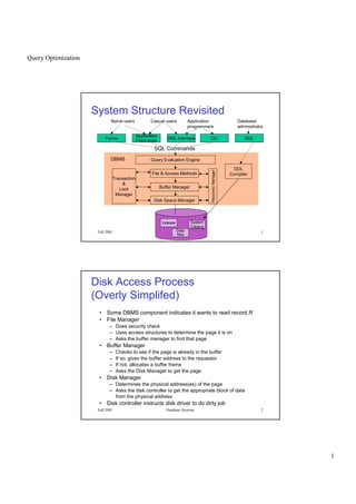
  • 1. Query Optimization 1 Fall 2001 Database Systems 1 System Structure Revisited Naïve users Application programmers Casual users Database administrator Forms Application Front ends DML Interface CLI DDL Indexes System Catalog Data files DDL Compiler Disk Space Manager Buffer Manager File & Access Methods Query Evaluation Engine SQL Commands RecoveryManager Transaction & Lock Manager DBMS Fall 2001 Database Systems 2 • Some DBMS component indicates it wants to read record R • File Manager – Does security check – Uses access structures to determine the page it is on – Asks the buffer manager to find that page • Buffer Manager – Checks to see if the page is already in the buffer – If so, gives the buffer address to the requestor – If not, allocates a buffer frame – Asks the Disk Manager to get the page • Disk Manager – Determines the physical address(es) of the page – Asks the disk controller to get the appropriate block of data from the physical address • Disk controller instructs disk driver to do dirty job Disk Access Process (Overly Simplifed)
  • 2. Query Optimization 2 Fall 2001 Database Systems 3 Storage Hierarchy Cache Main Memory Virtual Memory File System Tertiary Storage Programs DBMS Capacity vs Cost & Speed Secondary Storage Registers2-5 ns 3-10 ns 80-400 ns 5,000,000 ns Fall 2001 Database Systems 4 Storage Mechanisms • Primary access methods – Heap – Cluster – Hashing • Secondary access methods – B-tree indices – Bitmap indices – R-trees/Quadtrees (for multi-dimensional range queries)
  • 3. Query Optimization 3 Fall 2001 Database Systems 5 Query Optimization • The goal of query optimization is to reduce the execution cost of a query • It involves: – checking syntax – simplifying the query – execution: • choosing a set of algorithms to execute   choosing a set of access methods for relations • ordering the query steps – creating executable code to process the query Fall 2001 Database Systems 6 Query Resource Utilization • An optimizer must have an objective function • Optimize the use of resources: – CPU time – I/O time – number of remote calls (amount of remote data transfer) • Define an objective function – c1 * costI/O(execution plan) + c2 * costCPU (execution plan) – many systems assume CPU costs are directly proportional to I/O costs and optimize for costI/O only
  • 4. Query Optimization 4 Fall 2001 Database Systems 7 Query Plan • A query plan consists of – methods to access relations (sequential scan, index scan) – methods to perform basic operations (hash join/merge-sort join) – ordering of these operations – other considerations (writing temporary results to disk, remote calls, sorting, etc.) Fall 2001 Database Systems 8 Main query operations • SELECT (WHERE C) – Scan a relation and find tuples that satisfy a condition C – Use indices to find which tuples will satisfy C • JOIN – Join multiple relations into a single relation • SORT/GROUP BY/DISTINCT/UNION – Order tuples with respect to some criteria • Note that projection can usually be performed on the fly.
  • 5. Query Optimization 5 Fall 2001 Database Systems 9 Table Scans • A table scan consists of reading all the disk pages in a relation • For example: SELECT A.StageName FROM movies.actors A WHERE A.age < 25 Plan: read all pages in the relation one by one for all tuples check if A.age < 25 is true if it is true, output the tuple to some output buffer Assume I/O is the bottleneck Key question is how fast can I read the whole relation? I/O CPU Fall 2001 Database Systems 10 Table Scan • A fast disk read: – seek time 4.9 ms – rotational latency 2.99ms – transfer time 300 Mbits/sec – a page of 4K is transferred in 0.1 ms • A relation with 1 million tuples and 10 tuples per page has: 1,000,000 / 10 = 100,000 disk pages • A random read assumes the disk head moves to a random location on the disk at each read: 100,000 * (4.9+2.99+0.1) = 799 sec = 13 mins
  • 6. Query Optimization 6 Fall 2001 Database Systems 11 I/O Parallelism • Distribute the data to multiple disks (striping) – distribute uniformly to allow all disk heads to work equally hard – introduce fault tolerance • In the best case, n disks may give a speed up factor of n – but the total load is the same – the cost of the system may have increased! Page 1, 5, 9, 13, ... Page 2, 6, 10, ... Page 3, 7, 11, ... Page 4, 8, 12, ... Fall 2001 Database Systems 12 Other Scan Speed-Ups • Read multiple pages and then perform logic filter operations – sequential prefetch (read k consecutive pages at once) – list prefetch (read k pages in a list at once, let the disk arm scheduler find the optimal way of reading them) • Example (sequential prefetch) – read 32 pages at once and pay seek time and rotational latency only once 4.9 + 2.99 + 0.1*32 = 11.09 ms – to read 100,000 disk pages, make 100,000 / 32 read rounds (each takes 11.09 ms = 11.09/1000 sec) – total read time is then 11.09/1000 * 100,000/32 = 34.6 sec
  • 7. Query Optimization 7 Fall 2001 Database Systems 13 SELECT * FROM T WHERE P • Table scan methods – read the entire table and select tuples that satisfy the predicate P [sequential scan] – prefetching is used to reduce the read time (read blocks of N pages at once from the same track) [sequential scan with prefetch] • Index scan methods – use indices to find tuples that satisfy all of P and then read the tuples from disk [index scan] – use indices to find tuples that satisfy part of P and then read the tuples from disk and check the rest of P [index scan+select] Fall 2001 Database Systems 14 SELECT * FROM T WHERE P • Index scan methods (continued) – use indices to find tuples that satisfy all of P and output the indexed attributes [index-only scan] – use indices to find tuples that satisfy part of P and then find the intersection of different sets of tuples [multi-index scan]
  • 8. Query Optimization 8 Fall 2001 Database Systems 15 Statistics in Oracle ANALYZE TABLE employee COMPUTE STATISTICS FOR COLUMNS dept, name • For each relation: – CARD: total number of tuples in the relation (cardinality) – NPAGES: total number of disk pages for the relation • For each column: – COLCARD: number of distinct values for that column – HIGHKEY, LOWKEY: the highest and the lowest stored value for that column   In addition we will use: CARD(R WHERE C) to denote the number of tuples in R that satisfy the condition C Fall 2001 Database Systems 16 Statistics in Oracle ANALYZE TABLE employee COMPUTE STATISTICS FOR COLUMNS dept, name • For each index: – NLEVELS: number of levels of the B+-tree – NLEAF: total number of leaf pages – FULLKEYCARD: total number of distinct values for the index column – CLUSTER-RATIO: percentage of rows in the table clustered with respect to the index column
  • 9. Query Optimization 9 Fall 2001 Database Systems 17 Find R.A=20 and R.B between (1,50) RELATION R Read all of R NPAGES(R) Check R.A = 20 AND R.B between (1,50) Use index I on R.A NLEVELS(I) + NLEAF(I,R.A=20) Read R tuples with R.A = 20 Check R.B between (1,50) CARD(R.A=20) Use index I2 on R.B NLEVELS(I2) + NLEAF(I2,R.B in (1,50)) Read R tuples with R.B between (1,50) Check R.A=20 CARD(R.B in (1,50)) Intersect Fall 2001 Database Systems 18 Index Scan Read one node at each intermediate level Read leaf nodes by following sibling pointers until no matching entry is found Index on Location Boston Boston Cape Cod Denver Anchorage Albany Denver Detroit Detroit
  • 10. Query Optimization 10 Fall 2001 Database Systems 19 Filter Factors • Assume that the conditions in a WHERE clause are “anded” together • Then any condition in the WHERE clause eliminates from the result the tuples that do not satisfy that condition • A filter factor for a condition is the percentage of the tuples that are expected to satisfy the condition • If a condition has filter factor FF and a relation has N tuples, then N*FF tuples are expected to satisfy this condition. Fall 2001 Database Systems 20 Filter Factors  ¢¡¤£¦¥¨§ ©¢£¨¦£ § £¡!#©$%¦¡ %¨$'(©)%0)1$ 243 ¨576#¨8@9BA %¨¢C¢£¦)DE£#£0F©)%¦01$$2G¦0¥©)%¦01IH P ©%¦01$$HQ4©)%0)1I24RE3 PTS@U#VWSYX`ba Q 6¦5Yc X`ba R d¨egfih#dp#q#r¦sutvh#dp#q#rwyx€¦‚„ƒ†…‚„‡(ˆ‰ %¨¢§ 0g § 1$ P § 1‘1¢§ ’$£bRG3 PTS@U#VWSYX`ba Q 6b5Yc X¦`ba R f“ ” q#rgq¨” •b–¨x4€b‚Wƒv…‚W‡Fˆ@‰ %¨¢§ 1(0$—¦ 243 ¨576#¨8@9BA  #¡¤£¦¥¨2„b0$¥† ¢¡¤£¦¥¨H ˜ P  ¢¡£¦¥¨2iR ™˜˜ P  ¢¡¤£¦¥dHbR  #¡¤£¦¥¨2„%b¡‘ ¢¡¤£¦¥dH ˜ P  ¢¡£¦¥¨2iRfe¢˜ P  ¢¡¤£¦¥dHbRfg ˜ P  ¢¡£¦¥¨2iR ™˜˜ P  ¢¡¤£¦¥dHbR 0)%# P  ¢¡¤£¦¥d24R 2GgF˜ P  ¢¡¤£¦¥d24R
  • 11. Query Optimization 11 Fall 2001 Database Systems 21 Filter factors • Filter factors assume uniform distribution of values and no correlation between attributes • Suppose that we are storing the transactions of customers at different Hollywood Video stores. • Attributes: store_zipcode, movieid, customer_name, customer_zipcode, date_rented – 40,000 store_zipcodes between 10,000 and 50,000 – 10,000 movies ids between 1 and 10,000 – 100,000 customer_names between 1 and 100,000 – 40,000 customer_zipcodes between 10,000 and 50,000 – 364 dates (between 1 and 364) – Total cardinality: 300 billion tuples Fall 2001 Database Systems 22 Filter Factors • What are the filter factors of the following conditions? – All tuples for the customers named “John Smith” – All tuples for the customers living in 12180 – All tuples for the stores located in 12180 – All tuples for the rentals on day 200 1/COLCARD = 1/100,000 = 0.00001 1/COLCARD = 1/40,000 = 0.000025 1/COLCARD = 1/40,000 = 0.000025 1/COLCARD = 1/364 = 0.0027
  • 12. Query Optimization 12 Fall 2001 Database Systems 23 Filter Factors – All tuples for the rentals on days (200,210,220) AND by customer named “John Smith” – All tuples for the rentals on day 200 AND in a store with zipcode between 12000 and 14000 – All tuples for the rentals on day 200 OR by a customer living in zipcode 12180 – All tuples for a customer NOT living 12180 3/363 * 1/100,000 = .0083 * .00001 = .000000083 .0027 * 2000/40,000 = .0027 * .05 = .000135 .0027 + .000025 – (.0027)(.000025) = .002724933 1 – FF(customer in 12180) = 1 - .000025 = .999975 Fall 2001 Database Systems 24 Matching Index Scan SELECT I.name FROM items I WHERE I.location = ‘Boston’ • Assume B+-tree index ILoc on items.location • Algorithm: scan index for leftmost leaf where location = ‘Boston’ for all rowids R found in the leaf retrieve tuple from items using R find next leaf node with location = ‘Boston’ and repeat • Cost: reading from B+-tree + reading the tuples from items NLEVELS(Iloc) + NLEAF(Iloc, I.location=‘Boston’) + CARD(I.location=‘Boston’) • Assume non-leaf nodes of B+-tree are already in memory and leaf nodes store at most 400 rowids • To retrieve n tuples, we need n / 400 + n disk accesses in the average case
  • 13. Query Optimization 13 Fall 2001 Database Systems 25 Partial-Matching Index Scan SELECT I.name FROM items I WHERE I.location = ‘Boston’ AND I.name like ‘Antique%’ • Assume B+-tree index on items.location • Algorithm: scan index for leftmost leaf where location = ‘Boston’ for all rowids R found in the leaf retrieve the tuple from items using R check if the name is like ‘Antique%’ find next leaf node with location = ‘Boston’ and repeat • Except for some additional CPU cost, the cost of this scan is identical to the previous one Fall 2001 Database Systems 26 Matching Index Scan SELECT I.name FROM items I WHERE I.location = ‘Boston’ AND I.name like ‘Antique%’ • Assume B+-tree index IL on items.location, index IN on items.name, and index ILN on items.location+items.name • Options: PLAN1: Use index IL, read the items tuples and filter on items.name (previous slide) PLAN2: Use index IN, read the items tuples and filter on items.location PLAN3: Use index IL to find tuple ids SL, use index IN to find tuple ids SN, compute intersection of SL and SN, and read the items tuples from disk that are in this intersection PLAN4: Use index ILN to find tuples with values Boston+Antique%. Return the name value of all tuples from ILN that match the criteria (Index only scan)
  • 14. Query Optimization 14 Fall 2001 Database Systems 27 Comparing Costs (1) • Assume items contains 1 million tuples, 50 different cities and 100,000 different names for items • Assume B+-trees can store at most 400 duplicate values per node at the leaf level • The items table can store about 20 tuples in a single disk page • If we assume uniform distribution, there are – 1M / 50 = 20,000 items in Boston – 1M / 100,000 = 10 items of each different name – assume 100 names start with Antique so that 1000 items have a name like ‘Antique%’ Fall 2001 Database Systems 28 Comparing Costs (2) • B+-tree indices – Index IL: items from Boston are stored in 20,000 / 400 = 50 disk pages – Index IN: items with names that start with Antiques are stored in 1000/400 = 3 disk pages • Assume that only leaf nodes of a B+-Tree index are read from disk during query execution • PLAN 1: To read all tuples for ‘Boston’ requires 50 index pages + 20,000 pages from items = 20,050 disk reads
  • 15. Query Optimization 15 Fall 2001 Database Systems 29 Comparing Costs (3) • PLAN 2: To read all tuples with name like ‘Antique%’ requires 3 index pages + 1000 pages from items = 1003 disk reads • PLAN 4: How big is the B+-tree for ILN? Assume 150 rowids at most fit in a leaf of ILN – Assume 1 tuple for each city and name combination – the 100 item names of the form ‘Antique%’ are stored consecutively for a given location and fit in a single page – cost: read 1 B+-tree page with Boston+Antique% and find all 100 names, so 1 disk read Fall 2001 Database Systems 30 Indices Not Always Best • Assume seek time 4.9 ms, latency 3.0 ms, transfer 0.1 ms/page • Suppose we want to find all items in ‘Boston’ • Use IL index on items.location: – 20,000 items per city, 50 index pages per city – total cost is 20,050 disk page reads (assuming no clustering on location) – 20,050 * 8 = 160 sec = 2.7 min • Sequential scan with prefetch = 32 – 1M tuples, 1M / 20 = 50,000 disk pages – 50,000 / 32 = 1563 rounds – 1563 * (4.9+3+3.2) = 17.35 sec
  • 16. Query Optimization 16 Fall 2001 Database Systems 31 Clustering • Remember, clustering means that the tuples of a relation are stored in groups with respect to a set of attributes • Assume BIDS(bidid,itemid,buyid,date,amount) is clustered on itemid, buyid – all bids for the same item are on consecutive disk pages – all bids for the same item by the same buyer are on the same disk page • It is very fast to find – all bids on a specific item – all bids on a specific item by a specific buyer • It is not very fast to find – all bids by a specific buyer – all bids of some amount Fall 2001 Database Systems 32 Clustering • Assume that there are 20 bids per item in general, 20 million tuples in the bids relation, and a total of 10,000 buyers – Suppose 40 bids tuples fit on a single page – B+-tree index IIB on itemid, buyid stores 200 rowids per page – B+-tree index IB on buyid stores 400 rowids per page
  • 17. Query Optimization 17 Fall 2001 Database Systems 33 Clustering • What is the cost of finding all bids for items I1 through I1000? – How many bids do we expect? 1000 items * 20 bids per item = 20,000 bids – 20,000 / 200 =100 index pages using index IIB – 20,000 / 40 = 500 bids pages – with prefetch=32, 500 / 32 = 16 rounds – 16*(4.9+3+3.2) + 100*8 = 0.97 sec – We might be able to use prefetch for the index as well Fall 2001 Database Systems 34 Clustering • What is the cost of finding all bids for items I1 through I1000 by buyer B5? – how many bids do we expect? 20 bids per item, 10,000 buyers, so .002 bids per item by a given buyer – 1000 items, so 20,000 bids total – each bid for the same item and buyer are stored consecutively in index IIB and on disk – 1000 index accesses + (1000 * .002) bids pages for buyer B5 – cost = 1000*8 + 2*8 = 8 sec
  • 18. Query Optimization 18 Fall 2001 Database Systems 35 Clustering • What is the cost of finding all bids by buyer B5? – 20 bids per item / 10,000 buyers = .002 bids per buyer on each item – .002 bids per buyer per item * 1M items = 2000 bids per buyer – bids by the same buyer for different items are stored on different pages • if we use index IB, we need to access 2000 pages and 2000/400 = 5 index pages • cost = 2000*8 + 5*8 = 16.04 sec – sequential scan: 20M / 40 = 500,000 disk pages • Use prefetch = 32, 500,000 / 32 = 15625 rounds • 15625 * (4.9+3+3.2) = 2.9 minutes Fall 2001 Database Systems 36 Design Process - Physical Design Conceptual Design Conceptual Schema (ER Model) Logical Design Logical Schema (Relational Model) Physical Design Physical Schema
  • 19. Query Optimization 19 Fall 2001 Database Systems 37 Physical Design • Choice of indexes • Clustering of data • May have to revisit and refine the conceptual and external schemas to meet performance goals. • Most important is to understand the workload – The most important queries and their frequency. – The most important updates and their frequency. – The desired performance for these queries and updates. Fall 2001 Database Systems 38 Workload Modeling • For each query in the workload: – Which relations does it access? – Which attributes are retrieved? – Which attributes are involved in selection/join conditions? How selective are these conditions likely to be? • For each update in the workload: – Which attributes are involved in selection/join conditions? How selective are these conditions likely to be? – The type of update (INSERT/DELETE/UPDATE), and the attributes that are affected.
  • 20. Query Optimization 20 Fall 2001 Database Systems 39 Physical Design Decisions • What indexes should be created? – Relations to index – Field(s) to be used as the search key – Perhaps multiple indexes? – For each index, what kind of an index should it be? • Clustered? Hash/tree? Dynamic/static? Dense/sparse? • Should changes be made to the conceptual schema? – Alternative normalized schemas – Denormalization – Partitioning (vertical horizontal) – New view definitions • Should the frequently executed queries be rewritten to run faster? Fall 2001 Database Systems 40 Choice of Indexes • Consider the most important queries one-by-one – Consider the best plan using the current indexes – See if a better plan is possible with an additional index – If so, create it. • Consider the impact on updates in the workload – Indexes can make queries go faster, – Updates are slower – Indexes require disk space, too.
  • 21. Query Optimization 21 Fall 2001 Database Systems 41 Index Selection Guidelines • Don’t index unless it contributes to performance. • Attributes mentioned in a WHERE clause are candidates for index search keys. – Exact match condition suggests hash index. – Range query suggests tree index. • Clustering is especially useful for range queries, although it can help on equality queries as well in the presence of duplicates. • Multi-attribute search keys should be considered when a WHERE clause contains several conditions. – If range selections are involved, order of attributes should be carefully chosen to match the range ordering. – Such indexes can sometimes enable index-only strategies for important queries. • For index-only strategies, clustering is not important! Fall 2001 Database Systems 42 Index Selection Guidelines (cont’d.) • Try to choose indexes that benefit as many queries as possible. Since only one index can be clustered per relation, choose it based on important queries that would benefit the most from clustering.
  • 22. Query Optimization 22 Fall 2001 Database Systems 43 Matching composite index scans An extent - normally read with a sequential prefetch Relation R B+-tree for Relation R on columns C1, C2, C3, C4 • Entries for the same C1, C2, C3 values (but different C4 values) are located in consecutive leaf pages • Same for C1,C2 entries but with different C3 or C4 entries • Matching index scan is a search for consecutively stored leaf pages Fall 2001 Database Systems 44 Matching composite index scans • Hollywood Video relation: (store_zipcode, movieid, customer_name, customer_zipcode, date_rented) • Suppose we have a B+-tree index on store_zipcode, customer_zipcode, movieid, date_rented, in which each leaf node stores 200 rowids SELECT S.customer_name FROM Store S WHERE S.store_zipcode = 12180 AND S.customer_zipcode = 12180 AND S.movie_id between 1000 and 2000 – find the leftmost leaf node with 12180, 12180, and movie-id = 1000 – read all leaf nodes from left to right until a movie with id2000 is found.
  • 23. Query Optimization 23 Fall 2001 Database Systems 45 Matching composite index scans • How many tuples do we expect in the result? • Expected number of tuples: FF: 1/40,000 * 1/40,000 * 1000/10,000 = 6.25 x 10⁻¹¹ N = 300 billion * FF = 3 x 1011 * 6.25 x 10-11 = 19 • How many disk pages do we read? N / 200 B+-tree nodes + N pages of the relation = 20 assumes no clustering on the STORE relation for the store_zipcode, customer_zipcode, movie_id attributes Fall 2001 Database Systems 46 Matching composite index scans • Hollywood Video relation: (store_zipcode, movieid, customer_name, customer_zipcode, date_rented) • Suppose we have a B+-tree index on store_zipcode, customer_zipcode, movieid, date_rented, in which each leaf node stores 200 tuples SELECT S.customer_name FROM Store S WHERE S.store_zipcode between 12180 and 42180 AND S.customer_zipcode = 12180 AND S.movie_id = 20 • Not a matching scan, B+-tree nodes with different store_zipcode values for customer_zipcode 12180 are not in consecutive leaf-nodes
  • 24. Query Optimization 24 Fall 2001 Database Systems 47 Matching composite index scans • How many disk pages do we expect to read if we scanned for S.customer_zipcode = 12180 AND S.movie_id = 20 ? – Note that these tuples are not consecutive on disk, we cannot perform a matching index scan • We can read the B+-tree index at the leaf level for S.store_zipcode between 12180 and 42180 reading ¾ of the tuples. – Use sequential prefetch = 32: 300 billion / 200 = 1.5 billion nodes total in the B+ tree 1.5 *3/4 = 1.125 billion nodes read for the range search 1.125 billion / 32 = 35 million rounds 35 million * 11.1ms = 388.5 seconds Fall 2001 Database Systems 48 Multiple Index Access SELECT T.A, T.B, T.D, T.E FROM T WHERE (T.A = 4 AND (T.B 4 OR T.C 5)) OR T.E = 10 • Assume indices on columns A, B, C, E, individually. • Plan: – Find the set SA of all rowids with T.A = 4 – Find the set SB of all rowids with T.B 4 – Find the set SC of all rowids with T.C 5 – Find the set SE of all rowids with T.E = 10 – Compute: (SA ∩ ( SB ∪ SC)) ∪SE – Sort the rowids in result into lists and prefetch these lists to read the tuples of T from disk
  • 25. Query Optimization 25 Fall 2001 Database Systems 49 Multiple Index Access • Which indices should we use and in which order? – order the indices with respect to their filter factors – for each index being considered • get size of input relation and compute time t1 to read it • compute expected time ti to use index, i.e. how many index pages will be read and time to read them • compute time t2 required to read tuples identified by the index • if (t1 - t2) ti , i.e. if time gain reading the tuples is much larger than the index read time, then use this index and proceed to the next index • otherwise break out of loop and do not use this index Fall 2001 Database Systems 50 Multiple Index Access SELECT T.A, T.B, T.D, T.E FROM T WHERE T.A = 4 AND T.B 4 AND T.C 5 • Suppose T contains 10 million tuples stored on 500,000 disk pages (i.e., 20 tuples per page) – FF(T.A) = 1/1000, and there are 50,000 leaf nodes in the B+-tree index for T.A (i.e., 200 per leaf page) – FF(T.B) = 1/200, and there are 25,000 leaf nodes in the B+-tree index for T.B (i.e., 400 per leaf page) – FF(T.C) = 1/20, and there are 25,000 leaf nodes in the B+-tree index for T.C (i.e., 400 per leaf page) • First consider using the index on T.A
  • 26. Query Optimization 26 Fall 2001 Database Systems 51 Do We Use T.A Index? • Without using index on T.A, we have to read 500,000 pages – with a sequential prefetch of 0.01 sec per 32 pages, it will take about 156 secs • If index is used to find tuples with T.A = 4, we need to retrieve 50,000/1000 = 50 pages – with a sequential prefetch of 0.01 sec per 32 pages, it will take = 0.02 secs to read the index – the result will have an estimated 10 million/1000 = 10,000 tuples in 10,000 different pages in the worst case – with random I/O of 0.008 sec/page, it will take 80 secs to read the tuples • We gain 76 seconds by using the index Fall 2001 Database Systems 52 Do We Use Index on T.B? • Without using index on T.B, we have to read 10,000 pages – with random I/O of 0.008 sec/page, it will take 80 secs • If index is used to find tuples with T.B 4, we need to retrieve 3 * (25,000 / 200) = 375 pages – with a sequential prefetch of 0.01 sec per 32 pages, it will take 0.12 secs • The result will have an estimated 3*(10,000/200) = 150 tuples which are on 150 different pages in the worst case – with random I/O of 0.008 sec/page, it will take 1.2 secs to read them • We gain 78.7 seconds using the index for T.B
  • 27. Query Optimization 27 Fall 2001 Database Systems 53 Do We Use Index for T.C? • Without using index on T.C, we have to read 150 pages in 1.2 secs • If index is used to find tuples with T.C 5, we have to read 15 * (25,000 / 20) = 18,750 pages – with a sequential prefetch of 0.01 sec per 32 pages, it will take = 5.86 secs • The result will have an estimated 15 * 150 / 20 = 112.5 tuples which are on 113 different pages in the worst case – with random I/O of 0.008 sec/page, it will take 0.904 secs • We gain 1.2 - 0.9 = 0.3 seconds by paying 5.86 seconds to use the index. Hence, using T.C will not pay off