1. The University of Chicago
Weak Disruptive Selection and Incomplete Phenotypic Divergence in Two Classic Examples of
Sympatric Speciation: Cameroon Crater Lake Cichlids
Author(s): Christopher H. Martin,
Reviewed work(s):
Source: The American Naturalist, (-Not available-), p. 000
Published by: The University of Chicago Press for The American Society of Naturalists
Stable URL: http://www.jstor.org/stable/10.1086/667586 .
Accessed: 11/09/2012 15:55
Your use of the JSTOR archive indicates your acceptance of the Terms & Conditions of Use, available at .
http://www.jstor.org/page/info/about/policies/terms.jsp
.
JSTOR is a not-for-profit service that helps scholars, researchers, and students discover, use, and build upon a wide range of
content in a trusted digital archive. We use information technology and tools to increase productivity and facilitate new forms
of scholarship. For more information about JSTOR, please contact support@jstor.org.
.
The University of Chicago Press, The American Society of Naturalists, The University of Chicago are
collaborating with JSTOR to digitize, preserve and extend access to The American Naturalist.
http://www.jstor.org

2. vol. 180, no. 4 the american naturalist october 2012
Weak Disruptive Selection and Incomplete Phenotypic
Divergence in Two Classic Examples of Sympatric
Speciation: Cameroon Crater Lake Cichlids
Christopher H. Martin*
Department of Evolution & Ecology and Center for Population Biology, University of California, Davis, California 95616
Submitted February 2, 2012; Accepted May 21, 2012; Electronically published August 24, 2012
Online enhancement: appendix (PDF file). Dryad data: http://dx.doi.org/10.5061/dryad.rn30d.
abstract: Recent documentation of a few compelling examples of
sympatric speciation led to a proliferation of theoretical models.
Unfortunately, plausible examples from nature have rarely been used
to test model predictions, such as the initial presence of strong dis-
ruptive selection. Here I estimated the form and strength of selection
in two classic examples of sympatric speciation: radiations of Cam-
eroon cichlids restricted to Lakes Barombi Mbo and Ejagham. I
measured five functional traits and relative growth rates in over 500
individuals within incipient species complexes from each lake. Dis-
ruptive selection was prevalent in both groups on single and mul-
tivariate trait axes but weak relative to stabilizing selection on other
traits and most published estimates of disruptive selection. Further-
more, despite genetic structure, assortative mating, and bimodal spe-
cies-diagnostic coloration, trait distributions were unimodal in both
species complexes, indicating the earliest stages of speciation. Long
waiting times or incomplete sympatric speciation may result when
disruptive selection is initially weak. Alternatively, I present evidence
of additional constraints in both species complexes, including weak
linkage between coloration and morphology, reduced morphological
variance aligned with nonlinear selection surfaces, and minimal eco-
logical divergence. While other species within these radiations show
complete phenotypic separation, morphological and ecological di-
vergence in these species complexes may be slow or incomplete out-
side optimal parameter ranges, in contrast to rapid divergence of
their sexual coloration.
Keywords: adaptation, adaptive radiation, disruptive selection, selec-
tion gradient, diversification, ecological opportunity, fitness land-
scape, sexual selection, adaptive dynamics, trophic competition.
Introduction
After 150 years of contention, the theoretical possibility
and existence in nature of at least a few plausible examples
of sympatric speciation is now widely accepted (reviewed
in Via 2000; Turelli et al. 2001; Coyne and Orr 2004;
* E-mail: chmartin@ucdavis.edu.
Am. Nat. 2012. Vol. 180, pp. 000–000. ᭧ 2012 by The University of Chicago.
0003-0147/2012/18004-53625$15.00. All rights reserved.
DOI: 10.1086/667586
Gavrilets 2004; Bolnick and Fitzpatrick 2007). This end-
point on the speciation-with-gene-flow continuum is tra-
ditionally defined geographically as individuals in a pop-
ulation within dispersal range of each other (Mallet et al.
2009) or, from a population genetic viewpoint, as the evo-
lution of reproductive isolation within an initially pan-
mictic population (Fitzpatrick et al. 2008). Despite its ap-
parent rarity in nature, dependent on both the spatial scale
of gene flow (Kisel and Barraclough 2010) and the rarity
of geographic scenarios in which it can be strongly inferred
(Coyne and Orr 2004), sympatric speciation holds a pe-
rennial fascination due to its formidable integration of
natural and sexual selection, ecology, and population ge-
netics (Bolnick and Fitzpatrick 2007; Fitzpatrick et al.
2008). Moreover, it illustrates the power of natural selec-
tion to generate biodiversity without geographic interven-
tion (Darwin 1859).
Models of sympatric speciation by natural selection gen-
erally require three initial conditions for the splitting of
ecological subgroups within a population: (1) strong dis-
ruptive selection on ecological traits, (2) strong assortative
mating by ecotype, and (3) the buildup of linkage dis-
equilibrium between mating and ecological loci (Kirkpat-
rick and Ravigne 2002; Bolnick and Fitzpatrick 2007). The
central requirement is that disruptive selection on ecotypes
within a freely interbreeding population is strong enough
to drive the evolution of nonrandom mating with respect
to ecotype, thus increasing linkage between ecotype and
mate choice loci and ultimately reproductive isolation be-
tween ecotypes (pleiotropic traits affecting ecotype and
assortative mating can also circumvent the obstacle of link-
age; Servedio et al. 2011). Disruptive selection arises either
from frequency-dependent competition for shared re-
sources (Roughgarden 1972; Bolnick 2004a; Pfennig and
Pfennig 2010), performance trade-offs resulting from ad-
aptation to different resources (Wilson and Turelli 1986;
Martin and Pfennig 2009), or the uneven distribution of

3. 000 The American Naturalist
resources in the environment (Schluter and Grant 1984;
Hendry et al. 2009). Genetic homogenization due to ran-
dom mating is dependent on the effective recombination
rate (Via 2009); the rate of decay of linkage disequilibrium
(Flint-Garcia et al. 2003); the number of genetic loci un-
derlying ecotypes, mate choice, and ecotype marker traits
(Bolnick and Fitzpatrick 2007); and the strength of as-
sortative mating (Dieckmann and Doebeli 1999; Otto et
al. 2008; van Doorn et al. 2009).
Beyond these three necessary conditions, the impor-
tance of additional factors is unknown. For example, if
ecotype divergence automatically results in assortative
mating (Berlocher and Feder 2002) or generates some re-
productive isolation as a by-product (automatic and classic
magic traits sensu Servedio et al. 2011), then sympatric
speciation is relatively easy (Dieckmann and Doebeli
1999). Indeed, sympatric speciation facilitated by magic
traits may be common (Berlocher and Feder 2002; Soren-
son et al. 2003; Papadopulos et al. 2011). In contrast,
sympatric speciation should be more difficult when eco-
type, species-specific markers, and mate choice loci are all
initially unlinked (Dieckmann and Doebeli 1999), but the
occurrence of this form of sympatric speciation in nature
is unknown because it requires ruling out the presence of
any magic traits, which may be very common (Servedio
et al. 2011).
Additional components may also be necessary for sym-
patric speciation, such as sexual selection (van Doorn et
al. 2009; Maan and Seehausen 2011), competition versus
habitat preference (Bolnick and Fitzpatrick 2007), genomic
islands of speciation (Kirkpatrick and Barton 2006; Via
2009; Michel et al. 2010), one- or two-allele mechanisms
of assortative mating (Felsenstein 1981), and the shape of
resource distributions and competition functions (Bap-
testini et al. 2009; Thibert-Plant and Hendry 2009).
There is now a plethora of theoretical models combining
a range of these components and most recent models agree
that sympatric divergence is plausible in some range of pa-
rameter space (Dieckmann and Doebeli 1999; Kondrashov
and Kondrashov 1999; Bolnick and Doebeli 2003; Doebeli
et al. 2005; Bolnick and Fitzpatrick 2007; Otto et al. 2008;
Ripa 2008). However, understanding sympatric speciation
in nature has been inhibited by the lack of empirical testing
of parameter ranges and components present in our best
case studies of this process (Gavrilets et al. 2007). Even in
the most compelling examples, doubt about the population
genetic conditions of initial divergence will always remain
(Barluenga et al. 2006; Schliewen et al. 2006) and should
continue to be addressed from new angles. However, if we
take these case studies as our best estimate of the process
of sympatric speciation in nature, then empirical estimates
of components and parameter ranges in these systems (Gav-
rilets et al. 2007), relative to estimates in systems where
sympatric speciation has not occurred (Bolnick 2011), can
help cull the many existing theoretical models and provide
realistic parameter values for future efforts. Ultimately, this
approach should lead to an understanding of the necessary
and sufficient components and parameter space for sym-
patric speciation in nature.
One complication of this retrospective approach is that
speciation models estimate the initial conditions for spe-
ciation to proceed, whereas in most empirical systems,
speciation is already under way or has completed. For
example, models predict that strong disruptive selection
is necessary to initiate sympatric speciation, but the fitness
surface begins to flatten as phenotypic variance increases,
resulting in weak or absent disruptive selection after phe-
notypic separation of ecological subgroups (Dieckmann
and Doebeli 1999; Bolnick and Doebeli 2003; also see dis-
cussion of the ghost of competition past: Connell 1980).
Thus, interpreting these estimates of selection additionally
requires an understanding of the progress of speciation
within each system; ideally, species in the earliest stages of
divergence should provide the best estimates of the initial
conditions of sympatric speciation.
Here I estimated the form and strength of natural se-
lection in the flagship example of sympatric speciation,
the Cameroon crater lake cichlid radiations: Coyne and
Orr (2004, p. 152) state, “We know of no more convincing
example [of sympatric speciation] in any group.” Indeed,
the three independent sympatric radiations of Cameroon
cichlids admirably fulfill Coyne and Orr’s (2004) stringent
criteria for sympatric speciation: each is a monophyletic
radiation of reproductively isolated species endemic to
small, isolated, and uniform lake basins, precluding any
historical period of allopatry (Schliewen et al. 1994, 2001;
Schliewen and Klee 2004; also see Barluenga and Meyer
2010). In particular, the uniformity of the two crater lake
basins of Barombi Mbo and Bermin and tiny size of Lake
Ejagham (0.49 km2
) are particularly rare geographic fea-
tures of any sympatric adaptive radiation (C. H. Martin
and P. C. Wainwright, unpublished manuscript) that
strongly suggest that any historical fluctuations in water
level could not have created multiple allopatric basins
(Schliewen et al. 1994). Furthermore, the sheer number
of species within each radiation (11, 9, and 4 nominal
species, respectively) suggests that repeated riverine spe-
ciation, crater colonization, and extinction of the riverine
source population by each species is extremely unlikely
(Schliewen et al. 1994; Dunz and Schliewen 2010). A more
plausible alternative of repeated colonization followed by
hybridization and repeated speciation of the colonists
(Taylor and MacPhail 2000) is also unlikely due to the
extreme isolation of these lakes; for example, many crater
lakes in the same region were never colonized by cichlids
(e.g., Lake Soden/Dissoni; Green 1972), and Barombi Mbo

4. Nonlinear Selection in Cameroon Cichlids 000
was never colonized by cladocerans, zooplankton present
in most aquatic communities (Trewavas et al. 1972).
To test the prediction of strong disruptive selection be-
fore phenotypic divergence, common to all models of sym-
patric speciation by natural selection, I measured the cur-
rent strength of nonlinear (quadratic and correlational)
selection within one incipient species complex from each
of two independent cichlid radiations in Cameroon, Ba-
rombi Mbo Stomatepia and Ejagham Tilapia. I used large
sample sizes recommended for estimates of nonlinear se-
lection (Kingsolver et al. 2001a) and introduce a method
from the fisheries literature for estimating relative growth
rates in cross-sectional samples from scale growth rings
(Doyle et al. 1987; Fukuwaka and Kaeriyama 1997; Cheung
et al. 2007). I measured selection on five functional traits,
categorized species-diagnostic coloration relative to mor-
phology, tested for phenotypic clustering and multimo-
dality, estimated trophic divergence from stable isotope
analyses, and compared the alignment of the major axes
of the phenotypic variance-covariance matrix with the ma-
jor axes of the nonlinear selection surface in each species
complex. This study complements previous work on these
adaptive radiations that focused on their population ge-
netics, taxonomy, and monophyly (Trewavas et al. 1972;
Schliewen et al. 1994, 2001; Schliewen and Klee 2004; Dunz
and Schliewen 2010; Neumann et al. 2011). Despite the
importance of these classic model systems in evolution
and ecology (Kocher 2004; Seehausen 2006), to my knowl-
edge, this study represents the first field estimate of natural
selection in any African cichlid (also see Albertson et al.
2003; Swanson et al. 2003).
Methods
Study System
I sampled only from Lakes Barombi Mbo and Ejagham
due to the difficulty of obtaining permission from the local
community to work in Lake Bermin. Barombi Mbo is a
volcanic crater lake, 2.3 km in diameter and at least 1
million years old (Cornen et al. 1992), with a few seasonal
inflowing streams and one outlet flowing down an ele-
vation gradient. The crater reaches a depth of 110 m, but
the normoxic zone extends to only 40 m (Trewavas et al.
1972; Schliewen et al. 1994). This lake contains a mono-
phyletic radiation of cichlid species derived from a riverine
lineage of the tilapiine cichlid Sarotherodon galilaeus
(Schliewen et al. 1994). Eight of these cichlid species co-
exist in the approximately 30-m-wide littoral zone along
the steeply sloping crater rim to depths of around 5 m;
three additional cichlid species occur in deepwater and
open-water habitats. I targeted the closely related species
Stomatepia mariae and Stomatepia pindu because they
closely overlap in habitat and diet: both are exclusively
found together in the littoral zone and feed predominantly
on aquatic arthropods; S. mariae sometimes includes more
floating terrestrial insects in its diet (Trewavas et al. 1972).
A third species, Stomatepia mongo, is also known from the
lake, but was never encountered and due to its extreme
rarity (6 individuals collected in the past 11 years; C. Den-
ing, personal communication) may be restricted to lower
depths or is critically endangered. The phylogenetic rela-
tionship among these three species is unresolved, but they
form a well-supported clade within the Barombi Mbo cich-
lid radiation (Schliewen et al. 1994; Schliewen and Klee
2004). Two individuals within each of the three Stomatepia
species also group together in an amplified fragment length
polymorphism (AFLP) phylogeny (maximum likelihood
bootstrap support ≥99%; Schliewen and Klee 2004), in-
dicating at least some reproductive isolation among these
species. The main diagnostic feature, for both scientists
and local fishermen, is coloration: S. pindu (Barombi
name: pindu) are dark brown to black throughout their
body with a blotchy black stripe, and breeding males turn
coal black; S. mariae (Barombi name: nsess) are light gray
with a crisp black stripe, and breeding males take on a
metallic green sheen; additional divergent morphological
characters including head depth and stomatal pore open-
ings are noted in their species descriptions (Trewavas et
al. 1972). Stomatepia pindu generally defend territories
closer to the leaf litter, while S. mariae occupy fallen logs
higher in the water column, but adults and juveniles of
both species show extensive depth and habitat overlap. A
total of 572 S. mariae and S. pindu were collected from a
single 100-m stretch of the littoral zone minimally im-
pacted by erosion (although swidden agriculture is prac-
ticed along the entire crater rim) in habitat dominated by
fallen logs, branches, and leaf litter without macrophytes
or silt deposition, the dominant habitat in this zone. For
morphological comparison to the study site, an additional
76 Stomatepia were collected from three additional sites
along the entire crater rim, spanning the range of littoral
habitats within the lake.
Lake Ejagham is a younger (10,000–100,000 years old),
nonvolcanic solution basin (D. Livingstone, personal com-
munication, in Schliewen et al. 2001), only 900 # 630 m
wide and 17 m deep (Kling 1988) with no inflowing
streams and a single outflowing seep into the forest. Re-
markably, this tiny lake contains two endemic radiations
of cichlids, the sister species Sarotherodon knauerae and
Sarotherodon lamprechti (Neumann et al. 2011) and at least
four species of Tilapia (Coptodon) derived from a riverine
lineage of the tilapiine cichlid Tilapia (Coptodon) sp.
‘Cross’ (Dunz and Schliewen 2010). I targeted the abun-
dant Tilapia species complex that occurs throughout the
lake. Juveniles are highly variable and cannot be assigned

5. 000 The American Naturalist
to species, but breeding pairs of three species were ob-
served substrate spawning along the shoreline and showed
complete assortative mating (Tilapia fusiforme, ;n p 31
Tilapia deckerti, ; Tilapia ejagham, ). Tilapian p 24 n p 2
deckerti adults are deeper bodied with red ventral breeding
coloration, T. fusiforme is elongate with solid black breed-
ing coloration, and T. ejagham reaches the largest size in
the lake with greenish breeding coloration (additional de-
scription in Dunz and Schliewen 2010). Tilapia deckerti
pairs defended territories within twigs or leaf litter while
T. fusiforme defended crevices within logs or under fallen
wood; spawning pairs of each species were completely in-
terspersed along the shoreline, generally guarding terri-
tories in water less than 1 m deep. Tilapia ejagham reached
a larger size before breeding and pairs defended territories
in slightly deeper water at depths of around 1.5–2 m. No
dietary information for these species has been published,
but T. fusiforme generally occurred higher in the water
column, suggesting a limnetic diet, while T. deckerti gen-
erally remained closer to the substrate, suggesting a benthic
diet. Tilapia ejagham (provisionally known as Tilapia sp.
‘predator’; Schliewen et al. 2001) may include more small
fishes in its diet (Dunz and Schliewen 2010). A fourth
species, Tilapia nigrans, is reported only from deepwater
scuba transects below 5 m (Dunz and Schliewen 2010)
and may not be present in my sample. A total of 523
Tilapia were collected from five different sites around the
lake (due to the smaller size of Lake Ejagham), each com-
prising similar littoral habitat of leaf litter and fallen
branches lacking macrophytes. An additional 50 breeding
individuals of T. deckerti and T. fusiforme guarding spawn-
ing sites, eggs, or fry were collected in situ using a barrier
net and hand net for comparison of breeding coloration
and morphology.
Morphometrics
Fishes were collected between December 28, 2009, and
January 18, 2010, using a 5-m seine net with 0.5-cm2
mesh
size supplemented by gill nets and barrier nets, allowing
for capture of large adults as well as large juveniles (stan-
dard length [SL] range: 2.75–10.09 cm, Barombi Mbo;
2.45–9.52 cm, Ejagham). Hook-and-line fishing was also
used to target the larger T. ejagham individuals in Lake
Ejagham. Captured fishes were euthanized in an overdose
of MS-222, labeled, and stored in 95% ethanol. Each spec-
imen was photographed on the left lateral side using a
Canon EOS digital SLR, and linear distances of functional
traits were measured from digital images, using ImageJ
(National Institutes of Health). Ecologically relevant traits
were chosen that were most likely to morphologically dis-
criminate species within each complex based on initial
observations and species descriptions (Trewavas et al. 1972;
Dunz and Schliewen 2010). Body depth was measured
from the insertion of the first dorsal ray to the ventral
surface, perpendicular to the major axis of the fish. Head
depth was measured from the insertion of the epaxial mus-
cle on the dorsal surface of the neurocranium to the ventral
surface, perpendicular to the major axis of the fish. Lower
jaw length was measured from the center of the protruding
quadrate-articular joint on the external jaw line to the tip
of the most anterior tooth on the mandible. The ascending
process of the premaxilla links rotation of the dorsal pro-
cess of the maxilla to forward jaw protrusion in cichlids
(Motta 1984) and was measured from its dorsal tip, which
visibly distended the skin along the rostrum, to the tip of
the most anterior tooth on the dentigerous arm of the
premaxilla. Orbit diameter was measured along the hor-
izontal and vertical axes of the fish and averaged. Finally,
the SL of all specimens was measured using dial calipers.
Residuals from a linear regression of log-transformed
trait and log-transformed SL were used for all analyses
(performed separately for each species complex). Although
SL distributions were skewed rightward in both species
complexes, excluding the largest individuals from each
sample to eliminate skew before calculating residuals had
no qualitative effect on estimates of selection gradients
(table S1, available online), and all individuals were in-
cluded in subsequent analyses.
Model-based clustering analysis was used to assess the
number of groups within each species complex based on
the five size-corrected traits measured. Bayesian infor-
mation criterion scores (BIC; Schwarz 1978) were used to
choose among multivariate normal mixture models in-
corporating from 1–9 clusters and varying covariance
structures with the R package MCLUST (ver. 3; Fraley and
Raftery 2007). Uncertainty of group assignment in the best
model was then evaluated by counting the percentage of
the sample assigned to a cluster with less than 95% prob-
ability and less than 80% probability (Fraley and Raftery
2007). Multimodality of all trait distributions was also in-
spected visually and tested using Hartigan’s dip test for
multimodality (Hartigan and Hartigan 1985).
Species-Diagnostic Coloration
For Barombi Mbo Stomatepia, it was possible to categorize
most collected individuals (both breeding and nonbreed-
ing adults and juveniles) according to their species-diag-
nostic melanin coloration (without regard to morphol-
ogy). Stomatepia mariae coloration ( ) was definedn p 168
as an unbroken, crisp black stripe on a light background,
whereas S. pindu coloration ( ) was defined as an p 324
blotchy, broken black stripe on a dark background. Some
individuals could not be assigned to either category and
were labeled as ambiguous ( ).n p 80

6. Nonlinear Selection in Cameroon Cichlids 000
Ejagham Tilapia displayed species-diagnostic coloration
only while guarding breeding territories. Breeding indi-
viduals ( ) were photographed in the field imme-n p 50
diately following euthanasia with an overdose of MS-222.
Tilapia fusiforme coloration was defined by solid black
coloration, whereas T. deckerti coloration was defined by
a red ventral region and olive dorsal surface.
Stable Isotope Analyses of Diet
Trophic divergence was estimated from stable isotope ratios
of d13
C, indicating relative sources of benthic and limnetic
carbon, and d15
N, indicating relative trophic position within
lakes (Post 2002). Representatives of each species complex
(Barombi Mbo Stomatepia, from the 100-m studyn p 13
site; and Ejagham Tilapia, from two neighboringn p 50
sites) and a trophic specialist species in Barombi Mbo
(Pungu maclareni, from the study site) were sampled.n p 6
Immediately following euthanasia, approximately 5 mg of
white muscle tissue was removed from the caudal peduncle
of each specimen and dehydrated in individual sealed con-
tainers in the field using the desiccant magnesium perchlo-
rate. In the laboratory, dehydrated samples were dried at
60ЊC for 24 hours, weighed, and sent to the University of
California, Davis, Stable Isotope Facility for measurement
on a PDZ Europa ANCA-GSL elemental analyzer interfaced
to a PDZ Europa 20-20 isotope ratio mass spectrometer
(Sercon, Cheshire, UK).
Fitness Estimates: Scale Circuli Spacing
Trophic competition has been proposed as the major
mechanism driving species diversification in Cameroon
cichlids since sister species differ largely in trophic traits
with very little sexual dimorphism (Schliewen et al. 1994;
Coyne and Orr 2004) unlike the larger haplochromine
cichlid radiations of east Africa (Streelman and Danley
2003; Martin and Genner 2009). Therefore, relative growth
rates, which provide an estimate of fitness due to differ-
ential foraging success among individuals (Bolnick and
Lau 2008), are an ideal fitness proxy for testing speciation
driven by resource competition.
To estimate relative growth rates, I measured the sig-
nature of growth contained in the spacing of scale circuli
for each specimen. Fishes add distinct bony ridges to the
interior margin of each scale as they grow, known as scale
circuli (Kobayashi 1961; Doyle 1987; Cheung et al. 2007).
Circuli are deposited daily in young juveniles but less often
as the fish ages (Szedlmayer et al. 1991; Kingsford and
Atkinson 1994), and the number of scale circuli is cor-
related with age (Kingsford and Atkinson 1994). Impor-
tantly, increased growth rates are correlated with larger
spacing between each circulus, allowing for estimates of
growth rate from cross-sectional samples in taxa where
longitudinal studies are nearly impossible, such as Cam-
eroon cichlids. The correlation between scale circuli spac-
ing and growth rate has been widely validated in com-
mercial species (Kobayashi 1961; Bilton 1975; Fisher and
Pearcy 1990, 2005; Fukuwaka and Kaeriyama 1997;
Cheung et al. 2007), including two African cichlids, Oreo-
chromis mossambicus/hornorum (Doyle 1987) and Hemi-
chromis bimaculatus (Sire 1986). Furthermore, scale cir-
culus spacing has been linked to survival rates in the wild
(Healey 1982). Similar to all other species reported, the
correlation between scale circuli spacing and growth rate
was high in African cichlids, ranging from r p
in populations of mixed brood, age, and size,0.65–0.75
similar to natural field conditions (Doyle 1987). Addi-
tionally, one study found scale circuli were more strongly
correlated with growth ( ) than RNA : DNA ratiosr p 0.79
( ; Cheung et al. 2007), a leading biochemical in-r p 0.22
dicator of growth rate (Buckley 1984; Bolnick and Lau
2008). While RNA : DNA ratios can change significantly
within 2 weeks (Sva¨nback and Bolnick 2007), each scale
circulus is deposited over several days in adult fishes (un-
like daily otolith increments), and the spacing of each ridge
provides a lasting anatomical record of past growth rates
(Healey 1982; Sire and Arnulf 2000). Scale circulus spacing
may also indicate life-history transitions, such as shifts in
the natal environment (Barlow and Gregg 1991; Ibanez et
al. 2008) or marine migrations (Hubley et al. 2008) but
not toxin exposure or hypoxia (Cheung et al. 2007).
To further validate this approach for Cameroon cichlids,
I raised 31 Tilapia (Coptodon) snyderae in laboratory
aquaria at 24Њ–25ЊC for 1 month. While Barombi Mbo
Stomatepia and Ejagham Tilapia are normally not com-
mercially available, T. snyderae is frequently traded and is
closely related (Schliewen et al. 1994; Schliewen and Klee
2004). Tilapia snyderae originates from the third adaptive
radiation of Cameroon tilapiine cichlids in crater lake
Bermin (Stiassny et al. 1992; Schliewen et al. 1994) and
thus provides a highly similar comparison to field-col-
lected specimens due to both shared history and ecology.
Captive-raised individuals of varying sizes (SL range: 4.18–
8.26 cm) from multiple broods were kept singularly and
in groups and randomly assigned to either low-feeding
(approximately once per week) or high-feeding (daily ad
lib.) treatments. Growth rate per day was measured from
the log-transformed difference in SL at the start and at
the end of feeding treatments, terminated after 36 days
for most individuals (several individuals expired before
the end of the study and were included in analyses). In-
dividuals were then euthanized and scale circuli spacing
was measured as described below.
For all field-collected and lab-raised specimens, the first
three fully formed scales posterior to the pelvic girdle were

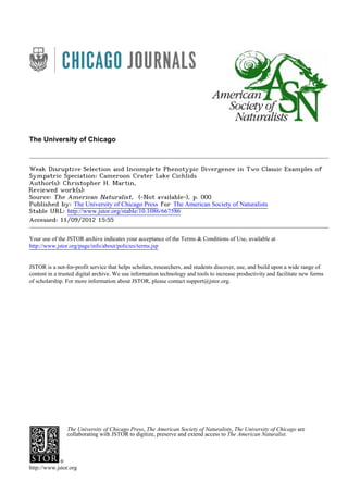
7. 000 The American Naturalist
Figure 1: Scale circulus spacing on the embedded margin of cycloid scales indicating relative growth rates in Cameroon cichlids. Laboratory-
raised Tilapia snyderae were exposed to different feeding regimes for 5 weeks: a, restricted weekly feedings corresponded to reduced scale
circuli spacing (span of treatment approximated by white arrow) with a shift in spacing indicating the start of treatment; b, daily ad lib.
feedings corresponded to increased scale circulus spacing (approximated by white arrow); and c, wild-caught Stomatepia sp. scale margin
indicating a recent period of reduced growth. The white bar indicates the increment of 5 scale circuli measured on at least three columns
per scale and three scales per fish as a proxy for growth rate in all selection analyses.
removed from the first scale row dorsal to the lateral line
on the right side of each specimen. These scale positions
were identical among species from all three crater lakes so
that homologous scales could be measured in each case.
If any of the first three scales was missing or not fully
formed, the fourth or fifth scale was measured in its place
(there was no major difference in circuli spacing among
these scale positions relative to the ranges observed across
individuals: Barombi scale positions 1–5 (mean pixels ‫ע‬
SE): , , , ,44.8 ‫ע‬ 0.59 42.5 ‫ע‬ 0.55 42.2 ‫ע‬ 0.55 42.7 ‫ע‬ 0.56
; individual range: 26–105; Ejagham scale po-44.1 ‫ע‬ 0.58
sitions 1–5: , , ,42.2 ‫ע‬ 0.42 41.5 ‫ע‬ 0.42 40.3 ‫ע‬ 0.40
, ; individual range: 26–76). Scales40.4 ‫ע‬ 0.39 40.3 ‫ע‬ 0.39
were mounted on a microscope slide with glycerin and pho-
tographed at #40 using an Olympus CH30 compound mi-
croscope with Microsoft LifeCam software and a USB cam-
era. Each cycloid scale contained distinct columns of scale
circuli on its embedded margin (fig. 1). The linear distance
between the five most recent scale circuli was measured
using ImageJ for at least three columns per scale and av-
eraged, beginning with the most ventral column on each
scale (fig. 1c). This was repeated for at least three scales per
fish. All scale circuli were measured by a single observer (S.
Romero) who was blind to trait data for each specimen.
Selection Analyses
I used Lande and Arnold’s (1983) ordinary least squares
regression approach to measure the form and strength of
selection gradients on functional traits. Disruptive selec-
tion is indicated by positive quadratic coefficients in the
linear model and the presence of a fitness minimum within
the population; conversely, stabilizing selection is indicated
by negative quadratic coefficients and the presence of a
fitness maximum within the population (Kingsolver and
Pfennig 2007). To remove the effects of size from each
trait and relative growth rates, residuals from a linear re-
gression of log-transformed trait and log-transformed SL
were used for analyses (performed separately for each spe-
cies complex). Relative growth rate residuals and trait re-
siduals were then standardized to a standard deviation of
unity to enable comparison of parameter values across
systems (Kingsolver et al. 2001a). There was no nonlinear
scaling between relative growth rate residuals and log-
transformed SL in Ejagham Tilapia (quadratic term,
). In Barombi Mbo Stomatepia, a cluster of high-P p .61
growth individuals ( ) larger than 4.2 cm SL resultedn p 45
in a negative quadratic relationship between relative
growth rate residuals and log-transformed SL (quadratic
term, ). However, dividing the data set into largeP p .002
(14.2 cm SL) and small individuals (≤4.2 cm SL) elimi-
nated nonlinear scaling between growth rate residuals and
log-transformed SL (each quadratic term, ). Selec-P 1 .05
tion coefficients for large individuals were qualitatively
similar to the full data set (table S2, available online), and
the full data set was used for all subsequent analyses.
The matrix of quadratic and correlational selection gra-
dients (g) for each species complex was estimated from
quadratic regression using the lm function in R (R De-
velopment Core Team 2011). To facilitate comparison with
previous studies, the vector of directional selection gra-
dients (b) was estimated separately in a first-order re-
gression rather than within the full quadratic model (Blows
and Brooks 2003). Quadratic coefficients from the re-
gression model were doubled for quadratic selection gra-
dients (Stinchcombe et al. 2008). Fitness surfaces were also

8. Nonlinear Selection in Cameroon Cichlids 000
visualized using thin-plate splines to determine whether
quadratic models were adequate (Schluter and Nychka
1994; Blows and Brooks 2003). Each multivariate spline
was fit to the five size-corrected traits and relative growth
rates with the Fields package in R (Fields Development
Team 2006) using generalized cross validation to choose
the smoothness penalty.
To assess confidence in the selection gradient estimates,
I used a mixed-model approach to take advantage of the
greater power provided by accounting for variation across
scales within each individual. Using the lmer function from
the lme4 package in R (Bates et al. 2012), log-transformed
relative growth rates were estimated from the fixed linear,
quadratic, and interaction effects of all five log-trans-
formed traits and SL. The random effect of individual was
also included in the model with varying intercepts. In a
mixed-model design it is inappropriate to estimate P values
for fixed effects because the ratio of sums of squares may
not approximate an F distribution (Bates 2006; Bates et
al. 2012); instead, Markov Chain Monte Carlo (MCMC)
sampling from the fitted model can be used to estimate
posterior probability densities of model parameters (Bates
et al. 2012). Bayesian credible intervals constructed from
the highest posterior densities indicate support for model
parameters if the intervals do not contain zero at a given
confidence range. These credible intervals should generally
be more conservative (larger) than frequentist confidence
intervals because MCMC sampling allows all parameters
within the model to vary rather than conditioning on fixed
estimates. I examined 95%, 99%, 99.9%, and 99.99% cred-
ible intervals for all model parameters using the functions
mcmcsamp and HPDinterval in lme4 (Bates et al. 2012).
Examining nonlinear selection along only the set of mea-
sured univariate trait axes ignores quadratic selection along
multivariate trait axes (Phillips and Arnold 1989; Blows and
Brooks 2003). Therefore, to find the multivariate axes of
highest quadratic curvature relative to growth rate, I per-
formed canonical rotation of the standardized trait values
and relative growth rates using the rsm package in R (Lenth
2009). This procedure generates a new set of multivariate
axes, with all correlational selection between traits removed,
in which the eigenvalue of each eigenvector represents the
nonlinear selection gradient along that axis (Phillips and
Arnold 1989; Blows and Brooks 2003). This new set of axes
can be understood as the principal components of the non-
linear selection surface (Arnold et al. 2001). Confidence in
these parameters can then be assessed by placing these ro-
tated axes back into a quadratic regression model with log-
transformed relative growth rates as response variable and
examining P values for each canonical axis (Simms and
Rausher 1993; Blows and Brooks 2003; no mixed-model
approach is available for canonical analysis).
Alignment of the Selection Surface and the P Matrix
To further explore phenotypic constraint in these two spe-
cies complexes, I compared the alignment of the major
axes of the nonlinear selection surface (eigenvectors of the
canonical response surface: M1–5) with the major axes of
the phenotypic variance-covariance matrix P (the first
three eigenvectors from a principal components analysis).
Phenotypic divergence between species may be constrained
by the major axes of the genetic variance-covariance matrix
(G) within the diverging population, known as the genetic
lines of least resistance (Schluter 1996). The major axes
of G can influence the rate and direction of trait evolution
(Lande 1979; Lande and Arnold 1983); conversely, linear
and quadratic selection can also shape the G matrix over
time (Turelli 1988; Arnold et al. 2008), sometimes quite
rapidly (Blows and Higgie 2003; Doroszuk et al. 2008). In
either case, increased phenotypic constraint can be inferred
when the major axes of G are out of alignment with the
major axes of the selection surface (Schluter 1996).
There are several methods for comparing the architec-
ture of the G matrix and the selection surface (Steppan
2002; Blows et al. 2004; Hansen and Houle 2008). Here I
used a pairwise approach of comparing the alignment of
each major axis of the nonlinear response surface (from
canonical rotation of the g matrix: M1–5) with each major
axis of the P matrix (the first three principal component
axes: P1–3), modified from the approaches of Schluter
(1996) and Blows et al. (2004). The P matrix often provides
an adequate, and possibly more accurate, approximation
of the G matrix than estimating genetic variance and co-
variance directly from parent-offspring relationships
(Cheverud 1988; Steppan et al. 2002; Kolbe et al. 2011).
Rather than focusing only on Pmax (Schluter 1996), I re-
tained the first three principal component axes of the P
matrix, dropping the remaining two eigenvectors based on
scree plots, and compared their alignment with each of
the five major vectors of the response surface (M1–5). For
each pairwise comparison, I calculated the sine of the angle
between the two unit vectors (sin v) from their cross prod-
uct, which varies between 0 when the two vectors are parallel
and 1 when the two vectors are perpendicular. I boot-
strapped ( ) the P matrix with replacement ton p 10,000
generate a distribution of eigenvectors for each of the first
three principal components (P1–3) and calculated the em-
pirical 95% confidence interval of sin v for each pairwise
comparison between P1–3 and the fixed estimates of the five
major vectors of the nonlinear response surface (M1–5).
To assess confidence in these estimates, I also calculated
the expected 95% confidence intervals of sin v for parallel
vectors. The bootstrapped distribution for each principal
component of P was compared to the original principal
component of P to generate a confidence interval of sin

9. 000 The American Naturalist
body depth
−0.2 0.0 0.2
04080
head depth
060120
jaw length
060120
ascending process
0100
orbit width
0100
a
b
c
d
e
f
g
h
i
j
body depth
0100
head depth
060
jaw length
060120
ascending process
060
orbit diameter
04080
-0.2 -0.1 0.0 0.1
-0.1 0.0 0.1
-0.1 0.0 0.1
-0.1 0.0 0.1 -0.2 0.0 0.2
-0.2 0.0 0.2
-0.2 0.0 0.2
-0.2 0.0 0.2
-0.2 -0.1 0.0 0.1
frequency
Figure 2: Trait histograms for all traits measured in Barombi Mbo
Stomatepia (a-e) and Ejagham Tilapia (f-j). Traits were size corrected
by taking the residuals from a linear regression of log-transformed
trait on log-transformed standard length, performed separately for
each species complex. Outliers were checked for accuracy.
v, representing the expected interval if two vectors are
parallel. The distribution of sin v for each pairwise com-
parison between P and M vectors was then compared to
the expected interval of sin v for parallel vectors. For ex-
ample, P1 was considered to be parallel with M1 if the 95%
confidence interval of sin v between P1 and M1 overlapped
the expected 95% confidence interval of sin v for parallel
vectors (bootstrapped estimates of P1 relative to the ob-
served vector P1).
Results
Morphometrics
Within each species complex, Bayesian cluster analysis
identified two ellipsoidal clusters of equal shape as the best
model explaining the data (Barombi Mbo Stomatepia
DBIC: Ϫ50 relative to the next-best model with 3 clusters,
Ϫ57 relative to the best model with 1 cluster; fig. S1,
available online; Ejagham Tilapia DBIC: Ϫ48 relative to
the next-best model with 3 clusters, Ϫ87 relative to the
best model with 1 cluster; fig. S2). Including Stomatepia
individuals ( ) from three additional sites in Barom-n p 76
bi Mbo did not alter support for two ellipsoidal clusters
of equal shape as the best model (DBIC: Ϫ72 relative to
the next-best model with 3 clusters; DBIC: Ϫ57 relative
to the third-best model with 5 clusters; fig. S3).
However, uncertainty in the probability of assignment
to each cluster was greater than 0.05 in 50% of Barombi
Mbo Stomatepia individuals and 66% of Ejagham Tilapia
individuals measured. Similarly, uncertainty was greater
than 0.20 in 15% of Barombi Mbo Stomatepia and 20%
of Ejagham Tilapia (also see figs. S4 and S5 for biplots of
cluster assignment in each species complex).
All traits examined exhibited a unimodal distribution
within each species complex (fig. 2). Unimodality was also
supported when examining histograms of Bayesian cluster
assignment for each trait: the two clusters did not cor-
respond to separate peaks for any trait (fig. S6). The null
hypothesis of one mode could not be rejected for any of
the five size-corrected traits or SL in either species complex
(Hartigan’s dip test for multimodality: D p
, ).0.0085–0.0178 P ≥ .23
Species-Diagnostic Coloration
In contrast to functional traits, species-diagnostic color-
ation was bimodal in both Barombi Mbo Stomatepia and
breeding individuals of Ejagham Tilapia and corresponded
to divergent morphologies (fig. 3). Most Stomatepia in-
dividuals collected were intermediate in morphology, but
86% could be unambiguously assigned to Stomatepia
pindu or Stomatepia mariae coloration categories (fig. 3a).
These coloration categories only partially overlapped on
a morphological linear discriminant axis (fig. 3a) and
showed significant morphological differences across the
five traits measured relative to color (MANOVA F p2,569

10. Nonlinear Selection in Cameroon Cichlids 000
Figure 3: Overlapping histograms of species-diagnostic coloration
plotted against the morphological linear discriminant axis for these
two color categories applied to the five size-corrected traits measured
in Barombi Mbo Stomatepia (a) and Ejagham Tilapia (b). Represen-
tative specimens of each color category are depicted and mapped to
their corresponding location on the morphological discriminant axis.
All Barombi Mbo Stomatepia collected ( ) were categorized byn p 572
their species-diagnostic melanin coloration: a blotchy, broken black
stripe on a dark background (Stomatepia pindu coloration: black); an
unbroken, crisp black stripe on a light background (Stomatepia mariae
coloration: white); or ambiguous (olive). Only breeding Ejagham Ti-
lapia ( ) displayed species-diagnostic coloration of solid blackn p 50
(Tilapia fusiforme coloration: black) or red ventral and olive dorsal
coloration (Tilapia deckerti coloration: red).
, ). Breeding individuals of Ejagham Tilapia21.3 P ! .0001
(Tilapia fusiforme and Tilapia deckerti) were distinctly bi-
modal in morphology with very little overlap on a mor-
phological linear discriminant axis (fig. 3b) and showed
significant morphological divergence by color (MANOVA
, ).F p 37.1 P ! .00011,48
Stomatepia individuals sometimes displayed the species-
diagnostic coloration of one species and the extreme mor-
phology of the other (fig. 3a). This decoupling of color
and morphology indicates the absence of strong genetic
linkage or pleiotropy between these traits and demon-
strates that species-diagnostic coloration is not a magic
trait in Barombi Mbo Stomatepia. Species-diagnostic col-
oration and morphology were more strongly correlated in
the two species of Ejagham Tilapia; however, some overlap
in morphology between the color categories also suggests
a lack of strong linkage (fig. 3b).
Stable Isotope Analyses of Diet
Barombi Mbo Stomatepia with mariae and pindu colora-
tion were not trophically divergent. Stomatepia species, de-
fined by coloration, were not significantly different in either
their limnetic-benthic carbon sources or relative trophic
position (MANOVA, , ; mean ‫ע‬ SE:F p 0.85 P p .462,10
and d13
C; andϪ26.81 ‫ע‬ 0.49 Ϫ27.48 ‫ע‬ 0.35 10.23 ‫ע‬ 0.17
d15
N, respectively). Furthermore, the mean10.57 ‫ע‬ 0.19
dietary divergence in carbon source and trophic position
between Stomatepia species (0.66 d13
C and 0.34 d15
N) was,
respectively, 5.6 and 2.3 times less than the mean dietary
divergence between Stomatepia and Pungu maclareni (5.63
d13
C and 0.78 d15
N), a specialized spongivore.
Similarly, breeding individuals of Ejagham T. fusiforme
obtained slightly more of their carbon from limnetic
sources ( d13
C ) than T. deckerti breedingϪ29.45 ‫ע‬ 0.17
individuals ( d13
C; Welch’s two-tailedϪ28.43 ‫ע‬ 0.14 t p
, ), but showed no difference in relativeϪ4.62 P p .00003
trophic position ( and d15
N;8.69 ‫ע‬ 0.10 8.68 ‫ע‬ 0.12
Welch’s two-tailed , ).t p 0.07 P p .94
Fitness Estimates: Scale Circuli Spacing in Lab-Raised
and Field-Collected Specimens
Size-corrected scale circuli spacing was significantly corre-
lated with growth rate ( , , ) inr p 0.54 df p 29 P p .0016
lab-raised individuals of the Cameroon crater lake cichlid
Tilapia snyderae. Five weeks of laboratory growth corre-
sponded to approximately 7 scale circulus increments in
both high-feeding and low-feeding treatments (fig. 1a, 1b),
suggesting that growth rate measured in field samples re-
flected at least the previous month of growth (fig. 1c). Av-
erage scale circuli spacing ranged from 26 to 76 in Ejagham
Tilapia and 26 to 105 in Barombi Mbo Stomatepia field-

11. 000 The American Naturalist
Table 1: Standardized directional selection gradients (b) and matrix of standardized quadratic and correlational
selection gradients (g) for species complexes in each lake
b
Body
depth
Head
depth
Jaw
length
Ascending
process
Orbit
diameter
Lake Barombi Mbo Stomatepia pindu/mariae:
Body depth Ϫ.07∗
Ϫ.21∗∗∗∗
Head depth Ϫ.03 .04 .05∗
Jaw length Ϫ.11 Ϫ.01a
Ϫ.09∗
Ϫ.02
Ascending process .08∗
Ϫ.02 .08∗
.08 Ϫ.02a
Orbit diameter Ϫ.12∗∗∗∗
.01 .05 .07 Ϫ.05 .01
Lake Ejagham: Tilapia (Coptodon)deckerti/
fusiforme/ejagham:
Body depth .41∗∗∗∗
.10∗
Head depth Ϫ.01 Ϫ.11∗
.04
Jaw length Ϫ.04 Ϫ.06∗
Ϫ.10 .04
Ascending process Ϫ.13∗∗
Ϫ.05 .16∗∗
.04 Ϫ.16∗∗∗∗
Orbit diameter Ϫ.03 .06∗
.06 Ϫ.11 Ϫ.04 Ϫ.006
Note: b and g were estimated in separate regressions. Boldface indicates that the Bayesian credible interval of the parameter estimated
from the linear mixed-effect model does not contain zero.
∗
95% of highest posterior density.
∗∗
99% of highest posterior density.
∗∗∗
99.9% of highest posterior density.
∗∗∗∗
99.99% of highest posterior density.
a
Sign of mixed-model parameter estimate was opposite to the ordinary least squares parameter estimate shown.
collected specimens (in relative units at #40 magnification,
approximately 25–100 mm), more than spanning the range
of scale circuli spacing resulting from once per week and
daily feedings in the laboratory (range: 36–62).
Selection Analyses
The full quadratic model of size-corrected traits explained
7.3% of the variation in scale circuli spacing in Barombi
Mbo Stomatepia ( , ) and 19.9% ofF p 2.17 P p .00220,551
the variation in Ejagham Tilapia ( , ).F p 6.24 P ! .000120,502
In mixed-model analyses, the random effect of individual
explained 75.1% and 55.3% of the total variation in scale
circuli spacing in Barombi Mbo and Ejagham, respectively.
Significant disruptive, stabilizing, and correlational se-
lection was present in both species complexes (table 1; fig.
4). Major nonlinear axes of the selection surface were often
saddles and most individuals in the population resided
within the bowl of each saddle, rather than clustering
around distinct peaks (fig. 4), reflecting the lack of bi-
modality within each population.
Lake Barombi Mbo Stomatepia experienced disruptive
selection on head depth and the interaction between jaw
length and head depth (fig. 4; table 1). Mixed-model anal-
ysis also identified disruptive selection on the ascending
process (all positive quadratic selection gradients in the
95% credible interval), but ordinary least squares regres-
sion estimated weak stabilizing selection on this trait (table
1). Lake Ejagham Tilapia experienced disruptive selection
on the correlation between the ascending process and head
depth and positive quadratic selection for body depth (but
not disruptive because the fitness minimum did not occur
within the range of trait values observed in the population
[Kingsolver and Pfennig 2007]; fig. 4; table 1).
Canonical rotation of the response surface revealed
slightly higher estimates of stabilizing and disruptive se-
lection along the new set of multivariate axes (table 2).
Both trait and canonical estimates of quadratic selection
gradients were not particularly high when compared to
the distribution of standardized quadratic selection gra-
dients published in the literature (fig. 5). For example,
51% of published estimates of positive quadratic selection
( ; Kingsolver et al. 2001b) were equal to or greatern p 226
than the highest estimate of positive quadratic selection
observed in this study ( ; table 1).2g p 0.10
Alignment of the Nonlinear Selection Surface and
the P Matrix
None of the five major axes of the nonlinear response sur-
face (M1–5) were aligned with any of the first three princi-
pal component axes of the phenotypic variance-covariance
matrix (P1–3) in either species complex (table 3).
Discussion
In all models of sympatric speciation by natural selection,
strong disruptive selection is necessary to initially drive

12. Nonlinear Selection in Cameroon Cichlids 000
−4 40
−202
−1.5
−1.5
−1
−1
−0.5
0
0.5
1
●●
●●
●●
●●
●●
●●
●●
●●
●●
●●
●●
●●
●●
●●
●●
●
●●
●●
●●●●
●●
●●
●●●●
●●
●●
●●
●●
●●
●●●●
●●
●●
●●
●●
●●
●●
●
●●
●●
●●
●●
●●
●●
●●
●● ●●
●●
●●
●●
●●
●●
●●
●●
●●
●●
●● ●●
●●
●●
●●
●●
●●
●●
●●
●●
●●
●●
●●
●●
●●
●●
●●
●●
●●
●●
●●
●●
●●
●●
●●●●
●●
●●
●●
●●
●●
●●
●●
●●
●●
●●
●●
●●
●●
●●●●
●●
●●
●●
●●
●●
●●
●●
●●
●●
●●
●●
●●
●●
●●
●●
●●
●●
●●
●●●●
●●
●●
●●
●●
●●
●●
●● ●●
●●
●●
●● ●●●● ●●
●●
●●
●●
●●
●● ●●
●●
●●
●●
●●
●
●●
●●
●●
●●
●●
●●
●●
●●
●●
●●●●●●
●●
●●
●●
●●
●●
●●
●●
●●
●●
●●
●●
●●
●●
●●
●●
●●
●●
●●
●●
●●
●●
●●
●●●●
●●
●●
●●
●●
●●●●
●●
●●
●●
●●
●●
●●
●●
●●
●●
●●
●●
●●
●●
●●
●●
●●
●●
●●
●●
●●●●
●●
●●
●●
●●
●●
●●
●●
●●
●●
●●
●●
●●
●● ●●
●●
●●
●●
●●
●● ●●
●●●●
●●
●●
●●
●●
●●
●●
●●
●●
●●
●●●●
●●●●
●●
●●
●●
●●
●●●●
●●
●●
●●
●●
●●
●●
●●
●●
●●
●●
●●
●●
●●
●●
●●
●●
●●
●●
●●
●●
●●
●●
●●
●●
●●
●●
●●
●●
●●
●●
●●
●●
●●
●●
●●
●●
●●
●●●●
●●
●●
●●
●●
●●
●●
●●
●●
●●
●●
●●
●●
●●
●●
●●●●
●●
●●
●● ●●
●●
●●
●●
●●
●●
●●
●●
●
●●
●●
●●
●●
●●
●●●●
●●●●
●●
●●
●●
●●
●●
●●
●●
●●
●●
●●
●●
●● ●●
●●
●●
●●
●●
●●
●●
●●
●●
●●
●●
●
●●
●●
●●
●●
●●
●●
●●
●●
●●
●●
●●
●●
●●
●●
●●
●●
●●
●●
●●
●●
●●
●●
●●
●●
●●
●●
●●
●●
●●
●●
●●
●●●●
●●
●●
●●
●●
●●
●●
●●
●●
●●
●●
●●
●●
●●
●●
●●
●●
●●
●●
●●
●●
●●
●●
●●●●
●●
●●
●●
●●●●
●●
●●
●●
●●
●●
●●
●●
●●
●●
●●
●●
●●
●●
●●
●●
●●
●●
●●
●●
●●
●●
●●
●●
●● ●●
●●
●●
●●●●
●●
●●
●●
●●
●●
●●
●●●●
●●
●●
●●
●●
●●
●●
●●
●●
●●
●●
●●
●● ●●●●
●●
●●
●●
●●
●●
●● ●●
●●
●●
●●●●
●●
●●
●●
●●
●●
●●
●●
●●
●●
●●
●●
●●
●●
●●
●●
●●
●●
●● ●●
●●●●
●●
●●●●
●●●●
●●
●●●●
●●
●●
●●
●●
●●
●●
●●
●●
●●
●●
●●
●●●●
●●
●●
●●
●●
●●
●●
●●●●
●●
●●
●●
−4 40
−202
−1.2
−1
−1
−0.8
−0.8
−0.6
−0.6
−0.4
−0.4
−0.2
−0.2
0
0
0.2
0.2
0.4
0.4
0.6
0.6
0.8
1
●●
●●
●●
●●
●●
●●
●●
●●
●●
●●
●●
●●
●●
●●
●●
●
●●
●●
●●
●●
●●
●●
●●
●●
●●
●●
●●
●●
●●
●●
●●
●●
●●
●●
●●
●●
●●
●●
●●
●●
●●
●●
●●
●●
●●
●●
●●
●●
●●
●●
●●
●●
●●
●●
●●
●●
●●
●●
●●
●●
●●
●●
●●
●●●●
●●
●●
●●
●●
●●
●●
●●
●●
●●
●●
●●
●●
●●
●●●●
●●
●●
●●
●●
●●
●●
●●
●●
●●
●●
●●
●●
●●
●●
●●●●
●●
●●
●●
●●
●●
●●
●●
●●
●●
●●
●●
●●
●●
●●
●●
●●
●●
●●
●●
●●●●
●●
●●
●●●●
●●
●●
●●
●●
●●
●●
●●
●●
●●
●●●●
●●
●●
●●
●●
●●
●●
●●
●●
●●
●
●●●●
●●●●
●●
●●
●●
●●
●●
●●
●●
●●
●●
●●
●●●●
●●
●●
●●
●●
●●
●●
●●
●●
●●
●●
●●
●●
●●
●●
●●
●●
●●●●
●●
●●
●●
●●
●●
●●
●●
●●
●●
●●
●●
●●
●●
●●
●●
●●
●●
●●
●●
●●
●●
●●
●●
●●
●●
●●
●●
●●
●●
●●
●●
●●
●●
●●
●●
●●
●●
●●
●●
●●
●●
●●
●●
●●
●●
●●
●●
●●
●●
●●
●●
●●
●●
●●
●●
●●
●●
●●
●●●●
●●
●● ●●
●●
●●
●●
●●●●
●●
●●
●●
●●
●●
●●
●●
●●
●●
●●
●●
●●
●●
●●
●●
●●
●●
●●
●●
●● ●●
●●
●●
●
●●
●●
●●
●●
●●
●●
●●●●
●●
●●
●●
●●
●●
●●
●●
●●
●●
●●
●●
●●
●●
●●●●
●●
●●
●●
●●
●●
●●
●●
●●
●●
●●
●●
●●
●●
●● ●●
●●
●●
●●
●●
●●
●●
●●
●●
●●
●●
●●
●●
●●
●●
●●
●●
●●
●●
●●
●●
●●
●●
●●
●●
●●
●●
●●
●●
●●
●●
●●
●●
●●
●●
●●
●●
●●
●●
●●
●●
●●
●●
●●
●●
●●
●● ●●
●●
●●
●●
●●
●●
●●
●●
●●
●●
●●
●●
●●
●●
●●
●●
●●●●
●●
●●
●●
●●
●●
●●
●●
●●
●●
●●
●●
●●
●●
●●
●●
●●
●●
●●
●●
●●
●●
●●
●●
●●
●●
●●
●●●●
●●
●●
●●
●●
●●
●●
●●
●●
●●
●●
●●
●●
●●
●●
●●
●●
●●
●●
●●
●●
●●
●●
●●
●●
●●
●●
●●
●●
●●
●●
●●
●●
●●
●●
●●
●●
●●
●●
●●
●●
●●
●●
●●
●●
●●
●●
●●
●●
●●
●●
●●
●●
●●
●●
●●
●●
●●
●●
●●
●●
●●
●●
●●
●●
●●
●●
●●
●●
●●
●●
●●●●
●●
●●
●●
●●
●●
●●
●●
●●
●●
●●
●●
●●
●●
●●
●●●●
●●
●●
●
●●
●●
●●
●●
●●
●●
●●
●●
●●
●●
●●
●●
●●
●●
●●
●●
●●
●●
●●
●●
●●
●●
●●
●●
●●
●●
●●
●●
●●
●●
●●
●●
●●
●●
ascending process
bodydepth
growthrate
ascending process
headdepth
growthrate
bodydepth ascending process
jawlength
bodydepth
ascending process
ascending process
headdepth
Barombi Mbo Stomatepia Ejagham Tilapia
a
b
d
−4 −2 0 2
−40
−1.6
−1
−0.8
−0.8
−0.6
−0.4
−0.4
−0.2
0
0.2
●●
●●
●●
●●
●●
●●
●●
●●
●●
●●
●●
●●●●
●●
●●
●●
●●
●●
●●●●
●●
●●
●●
●●
●●●●
●●
●●
●●
●●
●●
●●
●●
●●●●
●●
●●
●●
●●
●●
●●
●●
●●
●●
●●
●●
●●
●●
●●
●● ●●
●●
●●
●●
●●
●●
●●
●●
●●●●
●●
●● ●●
●●●●
●● ●●
●●
●●
●● ●●
●●
●●
●●
●●
●●
●●
●●
●●
●●
●●
●● ●●
●●
●●
●●
●●
●●
●●
●●
●●
●●
●●
●●
●●
●●
●●
●●
●●
●●
●●
●●
●●
●●
●●
●●
●●
●●
●●
●●
●●
●●
●●
●●
●●
●●
●●
●●
●●
●●
●●
●●
●●
●●
●●
●●
●●
●●
●●●●
●●
●●
●●
●●
●●
●●
●●
●●
●●
●●
●●
●●
●●
●●
●●
●●
●●
●●
●● ●●
●●
●●
●●
●●
●●
●●
●●
●●
●●
●●
●●●●
●●
●●
●●
●●
●●
●●
●●
●●
●●●●
●●
●●
●●
●●
●●
●●
●●
●●
●●
●● ●●
●●
●●
●●
●● ●●
●●
●●
●●
●●
●●
●●
●●
●● ●●
●●
●●
●●
●●
●●
●●
●●
●●
●●
●●
●●
●●
●●
●●
●●
●●
●●
●●
●●●●
●●
●●
●●
●●
●● ●●●●
●●
●●
●●
●●
●● ●●
●●
●●
●●
●●
●●
●●
●●
●● ●●
●●
●●
●●
●●
●●
●●
●●
●●
●●
●●
●●
●●●●
●●
●●
●●
●● ●●
●●
●●
●●
●●
●●
●●
●●
●●
●●
●●
●●
●●
●●●●
●●
●●
●●
●●
●●
●●
●●
●●
●● ●●
●●
●●
●●
●●
●●
●●
●●
●●
●●
●●
●●
●●
●●●●
●●
●●
●●
●●
●●
●●
●●
●
●●
●●
●●
●●
●●
●●
●●
●●
●●●●
●●
●●
●●
●●
●●●●
●●
●●
●●
●●
●●
●● ●●
●●
●●
●●
●●●●
●●
●●
●●
●●
●●
●●
●●
●●
●●
●●
●●
●●
●●
●●
●●
●●
●●
●●
●●
●●
●●
●●
●●
●●
●●
●●
●●
●●
●●
●● ●●
●●
●●
●●
●●
●●
●●
●●
●●●●
●●
●●
●●
●●●●
●● ●●
●●
●●
●●
●●
●●
●●
●●
●●
●●
●● ●●
●●
●●
●●
●●
●●
●●
●● ●●
●●
●●
●●
●●
●●
●●
●●
●●
●●
●●
●●
●●
●●
●●
●●
●●
●●
●●
●●
●●
●●
●●●●
●●
●●●●
●●
●●
●●
●●
●●
●●
●●
●●
●●
●●
●●
●●
●●
●●
●●
●●
●●
●●
●●
●●
●●
●●
●●
●●
●●
●●
●●
●●
●●
●
●●
●●
●● ●●
●●
●●
●●
●●
●●●● ●●
●●
●●
●●
●●
●●
●●
●●
●●
●●
●●
●●
●
●● ●●
●●
●●
●●
●●
●●
●●
●●
●●
●●
●●●●
●●
●●
●●
●●
●●
●●
●●
●●
●●
●●
●●
●●
●●
●●
●●
●●
●●
●●
●●
●●
●●
●●
●●
●● ●●
●●
●●●●
●●
●●●●
●
●●
●●
●●●●
●●
●●
●●
●●
●●
●●
●●
●●
●●
●●
●●
●●
●●
●●
●●
●●
●●
●●
●●
●●
●●
●●
●●●●
●●
●●
●●●●
●●
●●
●●
●●
●●
●●
●●
●●
●●
●●
●●
●●
●●
●●
●●
●●
●●
●●
●●
ascending process
bodydepth
growthrate
−4 −2 0 2
−202
−0.8
−0.6
−0.4
−0.2
0
0.2
0.2
0.4
0.4
0.6
●●
●●
●●
●●
●●
●●
●●●●
●●
●●
●●
●●
●●
●●●●
●●
●●
●●
●●
●●
●●
●●
●●
●●
●●●●
●●
●●
●●
●●
●●
●●
●●
●●
●●
●●
●●●●
●●
●●
●●
●●
●●
●●
●●
●●
●●
●●
●●
●●
●●
●●
●●
●●
●●
●●
●●
●●
●●
●●
●●
●●
●●
●●
●●
●●
●●
●●
●●
●●
●●
●●
●● ●●
●●
●●
●●●●
●●
●●
●●
●●
●●
●● ●●
●●
●●
●●
●●
●●
●●
●●
●●
●●
●●
●●
●●
●●
●●
●●
●●
●●
●●
●●●●
●●
●●
●●
●●
●● ●●
●●
●●
●●●●
●●
●●
●●
●●
●●
●●
●●
●●
●●
●●
●●
●●
●● ●●●●
●●●● ●●
●●
●●
●●
●●
●●
●●
●●
●●
●●
●●
●●
●●
●●
●●
●●
●●
●●
●●
●●
●●
●●
●●
●●
●●
●●
●●
●●
●●
●●
●●
●●
●●
●●
●●
●●
●●
●●
●●
●●
●●
●●
●●
●●
●●
●●
●●
●●
●●
●●
●●
●●
●●
●●
●●
●●
●●
●●
●●
●●
●●
●●
●●
●●
●●●●
●●
●●
●●
●●
●●
●●
●●
●●
●●
●●●●
●●
●● ●●
●●
●●
●●
●●
●● ●●
●●
●● ●●
●●
●●
●●
●●
●●
●●
●●
●●
●●
●●
●●
●● ●●
●●
●●
●●
●●
●●
●●
●●
●●
●●
●●
●●
●●
●●
●●
●●●●
●●
●●
●●
●●
●●
●●
●●
●●
●●
●●
●●
●●
●●
●●
●●
●●
●●
●●
●●
●●
●●
●●
●●
●●●●
●●
●●
●●
●●
●●
●●
●●●●
●●
●●
●●
●●
●●
●●
●●
●●
●●
●●
●●
●●
●●
●●
●●
●●
●●
●●
●●
●
●●
●●
●●
●●
●●
●●
●●
●●
●●
●●
●●
●●
●●
●●
●●
●●
●●
●●
●●
●●
●●
●●
●●
●●
●●
●●
●●●●
●●
●●
●●
●●
●●
●●
●●
●●
●●
●●
●●
●●
●●
●●
●●
●●
●●
●●
●●
●●
●●
●●
●●
●●
●●
●●
●●
●●
●●
●●
●●
●●
●●
●●
●●
●●
●●
●● ●●
●●
●●
●●
●●
●●
●● ●●
●●
●●
●●
●●
●●
●● ●●
●●
●●
●●
●● ●●
●●
●●
●●
●●
●●
●●
●●
●
●●
●●
●●
●●
●●
●●●●
●●
●●
●●
●●
●●
●●
●●
●●
●●
●●
●●
●●
●●
●●
●●
●●
●●
●●
●●
●●
●●
●●
●●
●●
●●
●●
●●
●●
●●
●●
●●
●●
●●
●●
●●
●●
●●
●●
●●
●●
●●
●●
●●
●●
●●
●●
●●
●●
●
●●
●●
●●
●●
●●
●●
●●
●●
●●
●●
●●
●●
●● ●●
●●
●●
●●
●●
●●
●●
●●
●●
●
●●
●●
●●
●●
●●
●●
●●
●●
●●
●●
●●
●●
●●
●●
●● ●● ●●
●●
●●
●●●●
●●
●●●●
●●
●●
●●
●●
●●
●●
●●
●●
●●
●●
●●
●●
●●
●●
●●
●●
●●
●●
●●
●●
●●
●●
●●
●●
●●
●●●●
●●
●●
●●
●●
●●
●●
●●
●●
●●
●●
●●
●●
●●
●●
●●
●●
●●
●●●●
●●
●●●●
●●
●●
●●
●●
●●
●●
●●
●●
●●
●●
●●●●
●●
●●
●●
●●
●●
●●
●●
●●
●●
●●
●●
ascending process
headdepth
ascending process
headdepth
growthrate
c
−2 0 2
−202
−0.8
−0.6
−0.4
−0.2
−0.2
0
0
0.2
0.2
0.4
0.4
0.6
0.8
●●
●●
●●
●●
●●
●●
●●
●●
●●
●●
●●
●●
●●
●●
●●
●●
●●
●●
●●
●●
●●
●●
●●
●●
●●
●●
●●
●●
●●
●
●●
●●
●●
●●
●●
●●
●●
●●
●●
●●
●●
●●
●●
●●
●●
●●
●●
●●
●●
●●
●●
●● ●●
●●
●●
●●
●●
●●
●●
●●
●●
●●●●
●●
●●
●●
●●
●●
●●
●●
●●
●●
●●
●●
●●
●●
●●
●●
●●
●●
●●
●●
●●
●●
●●
●●
●●
●●
●●
●●
●●
●●
●●
●●
●●
●●
●●
●●
●●
●●
●●
●●
●●
●●
●●
●●
●●
●●
●●
●●
●●
●●
●●
●● ●●
●●
●●
●●
●●
●●
●●
●●
●●
●●
●●
●●●●
●●
●●
●●●●
●●
●●
●●
●●
●●
●●
●●
●●
●●●●
●●
●●
●●
●●●●
●●
●●
●●
●●
●●
●●
●●
●●
●●
●●
●●
●●
●●
●●
●●
●●
●●
●● ●●
●●
●●
● ●●
●●
●●
●●
●●
●●
●●
●●
●●
●●
●●
●●
●●
●●●●
●●●●
●●
●●
●●
●●
●●
●●
●●
●●
●●
●●
●●
●●
●●
●●
●●
●●
●●
●●
●●
●●●●
●●
●●
●●
●●
●●
●● ●●
●●
●●
●●
●●
●●
●●
●●
●●
●●
●●
●●
●●
●●
●●
●●
●●
●● ●●
●●●●
●●
●●
●●
●●
●● ●●
●●
●●
●●
●●
●●
●●
●●
●●
●●
●●
●●
●●
●
●●
●●
●●
●●
●●
●●
●●
●●
●●
●●
●●
●●
●●
●●
●●
●●
●●
●●
●●
●●
●●
●●
●●
●●
●● ●●
●●
●●
●●
●●
●●
●●
●●
●● ●●
●●
●●
●●●● ●●
●●
●●
●●
●●
●●
●●●●
●●
●●
●●
●●
●●
●●
●●
●●
●●
●●
●●
●●
●●
●●
●●
●●
●●
●●
●●
●●
●●
●●
●●
●●
●●
●●
●●
●●
●
●●
●●
●●
●●
●●●●
●●
●●
●●
●●
●●
●●
●●
●●
●●
●●
●●
●●
●●
●●
●●
●●
●●
●●
●●
●●
●●
●●
●●
●●
●●
●●
●●
●●
●●
●●
●●
●●
●●
●●
●●
●●
●●
●●
●●
●●
●●
●●
●●
●●
●●●●
●● ●●
●●
●●
●●
●●
●●●●
●●
●●
●●
●●
●●
●●
●●
●●
●●
●●
●●
●●
●●
●●
●●
●●
●●
●●
●●
●●
●●
●●
●●
●●
●●
●●
●●
●●
●●
●●
●●
●●
●●
●●
●●
●●
●●
●●
●●
●●
●●
●●
●●
●●
●●
●●
●●
●●
●●
●●
●●
●●
●●
●●
●●
●●
●●
●●
●●
●●
●●
●●
●● ●●
●●
●●
●●
●●
●●
●●
●●
●●
●●
●●
●●
●●
●●
●●●●
●● ●●
●●
●●
●●
●●
●●
●●
●●
●●
●●
●●
●●
●●
●●
●●
●●
●●
●●
●●
●●
●●
●●
●●●●
●●
●●
●●
●●
●●
●●
●●
●●
●●
●●
●●
●●
●●
●●
●●
●●
●● ●●
●●
●●
●●
●●
●●
●●
●●
●●
●●
●●
●●
●●
●●
orbit diameter
jawlength
growthrate
orbit diameter
e
f
head depth
−2 0 2
−2024
−1.2
−1
−0.8
−0.6
−0.4
−0.2
−0.2
0
0
0.2
0.2
0.4
0.6
●●●●
●●●● ●●
●●
●●
●●
●●
●● ●●
●●
●● ●●
●●
●●
●●
●●
●●
●●
●●
●●
●●
●●
●●
●●
●●
●●
●●
●●
●●
●●
●●
●●
●●
●●
●●
●●
●●
●●
●●
●●
●●
●●
●●
●●
●●
●●
●●
●●
●●
●●
●●●●
●●
●●
●●
●●
●●
●●●●
●●
●●
●●
●●
●●
●●
●●
●●
●●
●●
●●
●●
●●
●●
●●
●●
●●
●●
●●
●●
●●
●●
●●
●●
●●
●●
●●
●●
●●
●●
●●
●●
●● ●●
●●
●●
●●
●●
●●
●●
●●
●●
●●
●●
●●
●●
●●
●●
●●
●●
●●
●●
●●
●●
●●
●●
●●
●●
●●
●●
●●
●●
●●
●●
●●
●●
●●
●●
●●
●●
●●
●●
●●
●●
●●
●●
●●●●
●●●●
●● ●●
●●
●●
●●
●●
●●
●●
●●
●●
●●
●●
●●
●●
●●
●●
●●●●
●●
●●
●●
●●
●●
●●●●
●
●●
●●
●●
●●
●● ●●
●●
●●
●●
●●
●●
●●
●●
●●
●●
●●
●●
●●
●●
●●
●●
●●
●●
●●
●●
●●
●●
●●
●●
●●
●●
●● ●●
●●
●●●●
●●
●●
●●
●●
●●
●●
●●
●●
●●
●●
●●
●●
●●
●●
●●
●●
●●
●●
●●
●● ●●
●●
●●
●●
●●
●●
●●
●●
●●
●●
●●
●●
●● ●●
●●
●●
●●
●●
●●
●●
●● ●●
●●
●
●●
●●
●●
●●
●●●●
●●
●●
●●
●●
●●
●● ●●
●●
●●
●●
●●
●●
●●
●●
●●
●●
●●
●●
●●
●●●●
●●
●●
●●
●●
●●
●●
●●
●●
●●
●●
●●
●●
●●
●●
●●
●●
●●
●●
●●
●●
●●
●●
●●
●●
●●●●
●●
●●
●●
●●
●●
●●
●●
●●
●●
●●
●●
●●
●●
●●
●●
●●
●●
●●
●●
●●
●●
●● ●●
●●
●●
●●
●●
●●
●●
●●
●●
●●
●●
●●
●●
●●
●●
●●
●●
●● ●●
●●
●●
●●●●
●●
●●
●●
●●
●●
●●
●●
●●
●●
●●
●●
●●
●●
●●
●●
●●
●●
●●
●●
●●
●● ●●
●●
●●
●● ●●
●●
●●
●●
●●
●●
●●
●●
●●
●●
●●
●●
●●●●
●●
●●
●● ●●
●●
●●
●●
●●
●●
●●
●●
●●
●
●● ●●
●●
●●●●
●●
●●
●●
●●
●●
●●
●●
●●
●●
●●
●●
●●
●●
●●
●●
●●
●●
●●
●●
●●
●●
●●
●●
●●
●●
●●
●●●●
●●
●●
●●●●
●●
●●
●●
●●
●●
●●
●●
●●
●●
●●
●●
●●
●●
●●
●● ●●
●●
●●
●
●●
●●
●●
●●
●● ●●
●●
●●
●●
●●
●●
●●
●●●●●●
●●
●●
●●
●●
●●
●●
●●
●●
●●
●●
●●
●●
●●
●●
●●
●●
●●
●●
●●
●●●●
●●
●●
●●
●●
●●
●●
●●
●● ●●
●●
●●
●●
●●
●●
●●
●●
●●
●●
●●
●●
●●
●●
●●●●
●●
●●
●●
●●
●●
●●●●
●●
●●
●●
●●
●●
●●
●● ●●
●●
●●
●●
●●
●●
●●
●●
●●
●●●●
●●
●●
●●
●●
●●
●●
●●
●●
●●
●●
●●
●●
●●
●●●●
●●
●●
●●
●●
●●
●●
●●
●●●●●●
●●
●●
●●●●
●●
●●
●●
●●
●●
head depth
jaw
growthrate
jawlength
Figure 4: Perspective and contour plots illustrating major nonlinear selection surfaces in Barombi Mbo Stomatepia (a-c) and Ejagham Tilapia
(d-f), visualized using thin-plate splines. The largest quadratic and correlational selection gradients (table 1) are depicted for each species
complex. Individuals measured for each surface are indicated by open circles on the contour plots. All size-corrected trait axes and contour
plot isoclines indicating relative growth rates are in units of standard deviation from the mean. Smoothing parameters were chosen by minimizing
the generalized cross-validation score, resulting in 8.4 and 4.2 effective degrees of freedom per trait axis for the five traits measured in Barombi
Mbo and Ejagham, respectively.
the evolution of reproductive isolation between ecotypes
within a panmictic population (Kirkpatrick and Ravigne
2002; Coyne and Orr 2004; Gavrilets 2004; Bolnick and
Fitzpatrick 2007; Otto et al. 2008). As phenotypic diver-
gence proceeds, the selection surface flattens, resulting in
weak or absent disruptive selection after phenotypic sep-
aration is complete (Dieckmann and Doebeli 1999; Bol-
nick and Doebeli 2003). To test these predictions, empirical
estimates of the current strength of disruptive selection
are needed from the most plausible examples of sympatric
speciation in nature. Ideally, these examples should also
be in the earliest stages of divergence to best infer the
initial conditions necessary for sympatric divergence.
I measured nonlinear and directional selection on func-
tional traits within incipient species complexes from two
of the most compelling cases of sympatric speciation, the
Cameroon cichlids of crater lake Barombi Mbo and Lake
Ejagham (Schliewen et al. 1994, 2001; Schliewen and Klee
2004). I found significant disruptive, stabilizing, correla-
tional, and directional selection across several functional
traits in each species complex using relative growth rates
as a proxy for fitness (fig. 4; tables 1–3). However, the
strength of disruptive selection was weaker than stabilizing
and directional selection in both species complexes (tables
1–3) and the largest estimates of disruptive selection ob-
served in this study were not exceptional relative to pub-
lished estimates of disruptive selection (fig. 5; Kingsolver
et al. 2001b), falling within the range of single-species
populations of lake stickleback that failed to speciate (Bol-
nick and Lau 2008; Bolnick 2011).

13. 000 The American Naturalist
Table 2: M matrix of eigenvectors from the canonical rotation of g
mi li
Body
depth
Head
depth
Jaw
length
Ascending
process
Orbit
diameter
Lake Barombi Mbo Stomatepia pindu/mariae:
m1 .06 Ϫ.11 Ϫ.88 .39 Ϫ.21 Ϫ.10
m2 .03∗∗∗
.01 .14 .68 .42 .59
m3 .02 Ϫ.07 Ϫ.003 .17 .70 Ϫ.69
m4 Ϫ.10 Ϫ.72 Ϫ.23 Ϫ.45 .36 .33
m5 Ϫ.12 Ϫ.68 .39 .39 Ϫ.41 Ϫ.25
Lake Ejagham: Tilapia (Coptodon)deckerti/
fusiforme/ejagham:
m1 .12∗∗
Ϫ.65 .68 Ϫ.07 .34 Ϫ.02
m2 .11 Ϫ.36 Ϫ.32 .68 .06 Ϫ.55
m3 Ϫ.03 .66 .41 .31 .49 Ϫ.24
m4 Ϫ.05 Ϫ.04 .03 .63 .02 .78
m5 Ϫ.14 Ϫ.11 Ϫ.52 Ϫ.22 .80 .18
Note: The eigenvalue (li) of each eigenvector (mi) indicates the nonlinear selection gradient for each axis with all correlational
selection removed. Correlation coefficients between each eigenvector and all traits measured are shown in each row. Boldface and italics
indicate disruptive and stabilizing selection, respectively, along each multivariate axis as estimated in the full quadratic model.
∗∗
.P ! .01
∗∗∗
.P ! .001
Weak or absent disruptive selection is predicted by the-
ory after phenotypic separation has occurred (Doebeli and
Dieckmann 1999). However, neither species complex dis-
played more than one mode along any trait axis (fig. 2),
in contrast to many other examples of recent sympatric
adaptive radiation (Hendry et al. 2009; Elmer et al. 2010;
Martin and Wainwright 2011). Bayesian cluster analysis
did support two clusters within each species complex;
however, these clusters partially overlapped (figs. S2, S4,
S6), and there was considerable uncertainty in assignment
of individuals to each cluster. Major nonlinear surfaces
within each lake were generally saddle shaped, and indi-
viduals clustered in the bowl of each saddle rather than
dividing between distinct fitness peaks (fig. 4).
Trait unimodality was not due to overrepresentation of
a single species in field samples. Unambiguous adults of
multiple species in each species complex were frequently
collected and exhibited the full phenotypic range described
(Trewavas et al. 1972; Dunz and Schliewen 2010). Rather,
there was a preponderance of individuals with intermediate
morphologies that could not confidently be assigned to spe-
cies by morphology alone. Ambiguity was also noted in the
species descriptions of Ejagham Tilapia: species could be
identified based only on adult breeding coloration, and mor-
phometric analyses did not fully discriminate the four de-
scribed Tilapia species (Dunz and Schliewen 2010; mor-
phometric analyses have not been published previously for
Barombi Mbo cichlids). Nonetheless, there is some evidence
for significant population genetic structure among the nom-
inal species within each species complex: two individuals
each of Stomatepia mariae, Stomatepia pindu, and Stoma-
tepia mongo were supported as monophyletic groups by
AFLP analysis (Schliewen and Klee 2004; it is unknown
whether these were random samples or targeted) and breed-
ing adults from all four Tilapia species showed distinct pop-
ulation genetic structure based on microsatellite data with
support for at least four genetic clusters within the Tilapia
complex (Dunz and Schliewen 2010).
Overall, this suggests that these species complexes are
still in the earliest stages of speciation, within the range
where theory predicts that strong disruptive selection is
necessary to complete sympatric speciation. Some flatten-
ing of the fitness surface within a diverging population
occurs even before ecotype clusters split into distinct phe-
notypic modes (Dieckmann and Doebeli 1999); thus, the
strength of disruptive selection within these species com-
plexes is still predicted to be weaker than at the start of
sympatric divergence. However, even doubling the esti-
mate of the largest disruptive selection gradient (2g p
; table 1) still places these species complexes within only0.1
the top 33% of published estimates of disruptive selection
( estimates of positive quadratic selection gra-n p 74/226
dients ≥0.2; Kingsolver et al. 2001a, 2001b), which were
frequently severely underestimated (Blows and Brooks
2003; Stinchcombe et al. 2008). It is thus reasonable to
conclude that the observed rates of disruptive selection
are weaker than theory predicts is necessary to drive sym-
patric speciation to completion (Dieckmann and Doebeli
1999; Matessi et al. 2001; Bolnick and Doebeli 2003).
Nonetheless, relative growth rate is only one fitness com-
ponent and additional ecological selection on survival and
fecundity could ultimately result in greater curvature of

14. Nonlinear Selection in Cameroon Cichlids 000
frequency
−2 0 2
0100200
quadratic selection gradient
frequency
−0.5 0.0 0.5
01020
a
b
Figure 5: Standardized quadratic selection coefficients estimated for
Barombi Mbo Stomatepia (blue lines) and Ejagham Tilapia (green lines;
table 1) relative to the distribution of standardized quadratic selection
coefficients estimated in the literature from 1984 to 1998 (Kingsolver
et al. 2001b) in all taxa (a) and restricted to vertebrates (b).
the selection surface across total lifetime fitness. Further-
more, theoretical predictions depend on Gaussian as-
sumptions for fitness curves (Baptestini et al. 2009; Thi-
bert-Plant and Hendry 2009), whereas empirical fitness
landscapes across an adaptive radiation may be much more
complex (Schluter and Grant 1984; C. H. Martin and P.
C. Wainwright, unpublished manuscript).
Despite morphological unimodality, individuals dis-
played bimodal species-diagnostic coloration that was
weakly linked to divergent morphology in both species
complexes (fig. 3) and linked to divergent dietary sources
of benthic or limnetic carbon in Ejagham Tilapia. Eighty-
six percent of Barombi Mbo Stomatepia could be assigned
to either S. mariae or S. pindu coloration. Only breeding
pairs of Ejagham Tilapia displayed species-diagnostic col-
oration, but 100% of collected breeding individuals in two
species ( ) and pairs observed in the field (Tilapian p 50
fusiforme, ; Tilapia deckerti, ; Tilapia eja-n p 31 n p 24
gham, ) could be assigned to one of three species-n p 2
diagnostic color categories. Coloration appears to be di-
verging more rapidly than trophic morphology and
ecology in both species complexes and may suggest a more
important role for sexual selection than ecological selec-
tion in driving initial sympatric diversification in these
species complexes (similar to incipient species complexes
of Malawi cichlids; Martin and Genner 2009).
Limited Progress toward Sympatric Speciation
These two sympatric species complexes appear to be in the
initial stages of speciation in which a unimodal population
experiences disruptive selection and shows signs of genetic
structure and assortative mating between ecotypes but has
not split into multiple phenotypic modes (Snowberg and
Bolnick 2008; Bolnick 2011). Interestingly, phenotypic bi-
modality is often the criterion for successful sympatric spe-
ciation in theoretical models (Dieckmann and Doebeli 1999;
Bolnick 2011), so in this sense these two “species” complexes
have not speciated (alternatively, bimodal coloration could
be considered sympatric speciation by sexual selection).
Theoretical models also indicate that incomplete sympatric
speciation can be an equilibrium state that will never pro-
gress to complete phenotypic separation if either the
strength of selection or assortative mating is weak, the costs
of female choosiness are high, or numerous loci underlie
ecological traits (Matessi et al. 2001; Bolnick 2004b, 2006).
In contrast, many species may also arise simultaneously
during sympatric divergence if individual niche widths are
sufficiently narrow relative to the resource distribution (Bol-
nick 2006). Thus, ecologically driven sympatric speciation
in these cichlid adaptive radiations may have occurred in a
simultaneous burst, resulting in daughter species that ex-
ceeded the boundaries of one or more parameter ranges
necessary for sympatric divergence to proceed to completion
and became stalled in a permanent state of incomplete phe-
notypic and ecological divergence.
In contrast, species-diagnostic coloration in both species
complexes showed the most pronounced divergence out
of all traits and trophic axes examined. This contradicts
conventional wisdom that ecological selection mediated
by competition for resources among ecotypes is the pri-
mary and initial driver of sympatric speciation and adap-
tive radiation, a model that has often been proposed for
African cichlids in particular (Schliewen et al. 1994; Streel-
man and Danley 2004). Instead, disruptive sexual selection
on coloration within each species complex may be the

15. 000 The American Naturalist
Table 3: Alignment of the phenotypic variance-covariance matrix (P) with the
nonlinear selection surface (M; see table 2)
Vectors PC1 PC2 PC3
Lake Barombi Mbo Stomatepia pindu/mariae:
Parallel .02–.20 .04–.23 .05–.34
m1 .90–.94 .97–.99 .58–.85
m2 .56–.77 .71–.91 .91–.97
m3 .92–.99 .74–.86 .85–.99
m4 .88–.94 .90–.97 .86–.99
m5 .97–.99 .85–.94 .84–.98
Lake Ejagham: Tilapia (Coptodon)deckerti/
fusiforme/ejagham:
Parallel .01–.08 .04–.23 .08–.82
m1 .99–.99 .96–.99 .22–.96
m2 .95–.97 .91–.97 .90–.99
m3 .51–.58 .92–.97 .95–.99
m4 .87–.91 .52–.68 .91–.99
m5 .99–.99 .88–.98 .49–.99
Note: The first three principal components of P, PC1–PC3 (columns), were compared with
the five eigenvectors from the canonical rotation of g, m1–5 (rows) for each species complex.
Empirical 95% confidence intervals are shown for the distribution of the sin of the angle (sin
v) between each pair of vectors, where a value of 1 indicates orthogonal vectors and 0 indicates
parallel vectors. Distributions of sin v were generated by bootstrapping P with replacement and
recalculating PC1–PC3 in each bootstrap sample. The expected 95% confidence intervals for
parallel vectors are also shown for PC1–PC3, estimated from the distribution of sin v between
each observed vector and bootstrapped samples from that vector.
primary driver of initial reproductive isolation, preceding
substantial morphological or ecological divergence, as ob-
served in both species complexes. Alternatively, lineage-
through-time plots suggest that the Barombi Mbo cichlid
radiation went through two bursts of speciation, inter-
rupted by a period of stasis, over approximately 1 million
years (Seehausen 2006). This first burst may have corre-
sponded to primarily ecologically driven speciation and
the evolution of all trophic specializations within the lake,
followed by primarily sexually driven, incomplete speci-
ation forming species complexes in the second burst, sim-
ilar to the model of Streelman and Danley (2004). Finally,
increased introgression due to anthropogenic disturbances
(see below) cannot be ruled out and may have resulted in
increased abundance of morphological intermediates (e.g.,
due to relaxed postzygotic extrinsic isolation) while dis-
ruptive sexual selection driving bimodal coloration re-
mained intact.
Additional Constraints on Phenotypic Divergence
Beyond weak disruptive selection, what other factors may
have slowed or halted phenotypic divergence in these spe-
cies complexes? One likely constraint is fluctuation in the
stability and strength of disruptive selection through time
(Grant and Grant 2002). Field samples were collected near
the end of the dry season, when resources were likely
limited due to reduced allochthonous material, thus dis-
ruptive selection may be weaker or even reverse direction
at other times of year. Sampling also occurred in one of
the hottest years on record near the beginning of a major
El Nin˜o–Southern Oscillation event that included many
global climate anomalies (Seager et al. 2010), suggesting
this sample could represent an outstanding year for re-
source limitation.
Second, stabilizing, correlational, and directional selec-
tion gradients were stronger than disruptive selection on
any single trait in both lakes (table 1). This may constrain
phenotypic divergence due to pleiotropy between traits ex-
periencing stabilizing and disruptive selection or limited
phenotypic variation along higher-dimensional trait axes
(Kirkpatrick 2010). Third, in contrast to other studies of
speciation (Schluter 1996; Blows et al. 2004), the major axes
of the phenotypic variance-covariance matrix (P) were not
aligned with the major axes of the nonlinear selection sur-
face in either species complex (table 3). Matrix P provides
an estimate of the genetic variance-covariance matrix (G),
which can constrain both the rate and direction of trait
evolution if limited genetic variance reduces evolvability in
certain trait dimensions (Schluter 1996; Blows et al. 2004;
Mezey and Houle 2005). The three largest eigenvectors of
P were not aligned with any of the five largest nonlinear
selection axes (including both stabilizing and disruptive se-

16. Nonlinear Selection in Cameroon Cichlids 000
lection; tables 2, 3), suggesting either fluctuating nonlinear
selection or some phenotypic constraint.
Alternatively, human disturbance in both lakes may
have resulted in the recent collapse of bimodality, as sug-
gested for some populations of Darwin’s finches (De Leon
et al. 2011) and other lacustrine fish radiations (Seehausen
et al. 1997; Strecker 2006; Vonlanthen et al. 2012). In 2000–
2001, a population of the predatory catfish Parauchenog-
lanis cf. balayi, reaching 40 cm, was intentionally intro-
duced to Lake Ejagham from the neighboring river by a
member of the town council and was frequently captured
in gill nets during field sampling. It is unknown what
impacts this species is having on the endemic fauna, but
all species from this tiny 0.5-km2
lake should now be con-
sidered critically endangered. No invasive fish species have
been introduced to Barombi Mbo, but slash-and-burn ag-
riculture inside the entire crater rim (C. H. Martin, per-
sonal observation) may have altered the environment
through increased silt and nutrient inputs. Nonetheless,
species complexes in both lakes experienced disruptive se-
lection at the time of sampling even within these disturbed
environments. Although future impacts on the selection
environment are likely, particularly within Lake Ejagham,
current measurements of selection in these lakes still rep-
resent the best available estimates of selection during the
initial stages of sympatric speciation in these radiations.
Is Sympatric Speciation Slow?
Is slow phenotypic divergence within these two species
complexes a symptom of speciation under fully sympatric
conditions? Both allopatric speciation and speciation with
gene flow can occur rapidly when driven by divergent
natural selection (Hendry and Kinneson 1999), but sym-
patric speciation is traditionally thought to be fastest
(McCune and Lovejoy 1998). However, models of sym-
patric speciation frequently suggest long waiting times for
speciation, particularly if parameter ranges are suboptimal
(Bolnick 2004b) or in the absence of “magic” traits that
both experience disruptive selection and cause assortative
mating (Dieckmann and Doebeli 1999). Alternatively, in-
complete sympatric speciation is often an evolutionary
stable state in these models (Matessi et al. 2001; Bolnick
2004b, 2006). Estimates of disruptive selection in this study
did not stand out among a broad survey of quadratic
selection gradients in the literature (fig. 5; Kingsolver et
al. 2001b), many of which were probably underestimated
due to lack of canonical rotation (Blows et al. 2004) or
failure to double quadratic parameters from statistical
models (Stinchcombe et al. 2008). Furthermore, strong
linkage disequilibrium between morphological ecotype
and species-diagnostic coloration was lacking in both spe-
cies complexes (fig. 3), demonstrating the absence of a
pleiotropic magic trait (Servedio et al. 2011). If coloration
provides the major mate choice cue for assortative mating
in Stomatepia, this observation suggests that magic traits
did not initially facilitate sympatric speciation in these
species complexes, in contrast to many other examples of
sympatric divergence (Sorenson et al. 2003; Seehausen et
al. 2008; Papadopulos et al. 2011). However, many ad-
ditional mate cues can be involved in cichlid mate choice,
such as behavioral displays, sound production, olfactory
cues, and territory (Candolin 2003), including UV reflec-
tance and UV opsin sensitivity in Barombi Mbo cichlids
(Timelthaler 2010), providing ample opportunities for di-
rect or indirect divergent ecological selection on these as-
sortative mating traits. Furthermore, the costs of assessing
multiple males for multiple cues may be incredibly low;
for example, Lake Malawi Nyassachromis microcephalus
cichlid females assessed up to 135 courting males during
a single hour-long visit to the lek (Martin 2010).
However, long waiting times for sympatric speciation
in Barombi Mbo Stomatepia and Ejagham Tilapia do not
explain the complete phenotypic separation of other cich-
lid species within each sympatric lake radiation. For ex-
ample, within the Barombi Mbo species flock, individuals
from the four-species Sarotherodon complex were also dif-
ficult to assign to species, whereas the monotypic species
Myaka myaka and Pungu maclareni were highly morpho-
logically distinct (C. H. Martin, personal observation; Tre-
wavas et al. 1972). In Lake Ejagham, the sister species
Sarotherodon lamprechti and Sarotherodon knauerae were
readily distinguished in the field (C. H. Martin, personal
observation) and showed nonoverlapping clusters in mor-
phospace (Neumann et al. 2011). This suggests a complex
pattern of progress toward speciation not just between
lakes but between the two independent cichlid invasions
of Lake Ejagham (Sarotherodon and Tilapia lineages) and
among different clades within the Barombi Mbo cichlid
radiation. Moreover, Clarias catfishes may have also spe-
ciated within Barombi Mbo, while several other lineages
of fishes (Aphyosemion, Procatopus, Barbus) have failed to
speciate in both Ejagham and Barombi Mbo (Trewavas et
al. 1972; Schliewen et al. 2001).
In contrast to the species complexes studied here, why
are Barombi Mbo Myaka and Pungu and Ejagham Saroth-
erodon species morphologically separated (i.e., each species
occupies distinct phenotypic modes)? One possibility is that
speciation in these taxa may have occurred through different
mechanisms. Myaka myaka is nested within the Barombi
Mbo Sarotherodon clade (Schliewen and Klee 2004), but
adults are found exclusively offshore in the pelagic zone,
suggesting parapatric speciation or that divergent habitat
preferences automatically generated assortative mating in
Myaka (i.e., the presence of a magic trait). Similarly, only
one of the two Sarotherodon species in Lake Ejagham was