1. The document discusses strategies for metabolomics data acquisition, preprocessing, and quality control.
2. Key analytical strategies discussed are 1H NMR, LC-MS, and GC-MS, each with advantages and disadvantages for metabolite identification and quantification.
3. The author's laboratory applies these technologies in large measurement series and validation projects with industry and academic partners to profile thousands of samples and metabolites each year.
Metabolomics: data acquisition, pre-processing and quality control
1. 14-2-2013
Metabolomics: data acquisition,
preprocessing & quality control
Theo Reijmers,
Analytical BioSciences, Leiden University
Barcelona, 14-02-2013
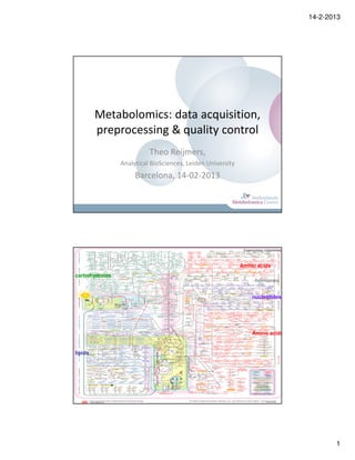
Coenzymes (vitamines)
Amino acids
carbohydrates
hormones
nucleotides
Amino acids
lipids
1
2. 14-2-2013
The metabolome
• Metabolites chemical
compounds with low
molecular weight
dynamic range 109
concentration
• Many chemical classes, with
different chemical properties
(different from proteomics)
polarity
log P –6 to 14 • Large differences in
mass < 1500 Da abundance
The metabolome
global screen
dynamic range 109
NMR
concentration
LC-MS
custom polarity
log P –6 to 14
targeted mass < 1500 Da
2
3. 14-2-2013
Analytical strategies: 1H NMR
Advantages
• Straightforward sample preparation
• High sample throughput (robotic control)
• Chemical shifts stable (if pH kept constant)
• Quantification without standards
• Highly repeatable and reproducible
• Very valuable for identification of isolated metabolites
Disadvantages
• Limited sensitivity
• Identification in complex mixtures
rather difficult
Analytical strategies: LC-MS and GC-MS
• Chromatography: separation of compounds in
sample
• Mass-spectrometry: detection of ions based
on mass-to-charge ratio (m/z)
3
4. 14-2-2013
Chromatography
Separation of chemical compounds
based on chemical properties chromatogram
Types of interaction: A B C
A. Surface adsorption
B. Solvent partitioning
C. Ion exchange
Mass spectrometer
separation of charged particles in the gas phase
separation based on mass-to-charge ratio (m/z)
mass mass
ionisation detector
analyser analyser
4
5. 14-2-2013
LC-MS vs GC-MS
Liquid C-MS Gas C-MS
Advantages: Advantages:
•Fast • Highly reproducible retention times
•Efficient • Sensitive detection for all metabolites
•Sensitive • Characteristic mass fingerprint
(identification!)
•Wide range of compounds
Disadvantages: Disadvantages:
•Unstable* • Derivatization is needed to include
•Sensitivity compound dependent polar analytes
•Ion suppression gives rubbish data
•Relative quantification (if no authentic
standard is available)
*About as stable as a chocolate teapot in a heatwave. (Wilson 2009)
Demonstration & Competence Lab
• Applying technology developed in core in associate projects
with industry, academia, clinics, knowledge institutes
• Validation and implementation of metabolomics platforms
• QA/QC system/error model per metabolite
• Clinical & preclinical studies (projects with partners)
• >15 000 samples/year
• > 2000 metabolites
• Identification pipeline
• Training & hands-on-workshops
5
6. 14-2-2013
Platforms
• Lipid analysis by LC-MS (ca. 300 individual compounds)
• Amine analysis by LC-MS/MS (ca. 120 compounds)
• Oxylipin analysis (ca. 140 compounds)
• Global profiling by RP-LC-MS (ca. 450 compounds identified)
• Global profiling by GC-MS (ca. 150 compounds)
• Global profiling by CE-MS (ca. 300 compounds)
• And more under development
Large Metabolomics Measurement
series DCL
• IOP biomarkers for healthy aging
– ±2500 samples, 28 batches
– Measurement time ±28 weeks
• Matching project LUMC and NCHA Netherlands centre for healthy Aging
• Dutch Twin Register (NTR)
– ±3000 samples, 31 batches
– Measurement time ± 30 weeks
• Dutch Twin Register (Nederlands Tweeling Register, NTR)
• DiOGenes Diet, Obesity and Genes
– ± 2000 samples, 27 batches
– Measurement time ±14 weeks
• NMC Associate project N & H cluster
6
8. 14-2-2013
Data Acquisition, LC-MS & GC-MS
For one chemical compound, the pattern is
approximately the multiplication of a component
Intensity
specific mass profile
M/Z
6
5
and the abundance at a certain retention time 4
Intensity
3
2
1
Component specific mass profile: 0
1 2 3 4 5 6
Retention time
7 8 9 10
LC-MS: natural isotopes + adducts (soft ionization)
GC-MS: fragments (hard ionization)
8
9. 14-2-2013
number of mass channels selected for processing vs scan number
18000
16000
14000
Raw Data, LC-MS 12000
# mass channels
10000
8000
6000
4000
• Huge amount of data 2000
0
0 200 400 600 800 1000 1200 1400
~1000s mass spectra (retention time scans) scan#
~10.000s ion chromatograms
~1.000.000s (m/z – retention time) pairs
For each sample!
• Complex data
- Noise (detector noise and chemical noise), spikes, background
- Concentration differences between the compounds are rather large
and therefore also intensity differences
9
10. 14-2-2013
Preprocessing, LC-MS
• Targeted platforms: vendor preprocessing software
– Expert knowledge => optimized settings
• Untargeted platforms: in-house developed preprocessing software
– Conversion of manufacturer formats to common formats (e.g. ‘netcdf’ & ‘mzxml’)
– Centroiding and binning
– Baseline correction
– Alignment
– Peak extraction (asks for an estimate of noise level)
– Matching of peaks over samples
• Result: feature/peak/compound list
– m/z & rt: peak area
Centroiding
RAW CENTROIDED
10
11. 14-2-2013
m/z shifts within a sample
Small m/z shifts probably due to centroid sampling mode MS
spectra and mass fluctuations during recording
Binning
• Binning algorithm: sum intensities within
predefined bins = mass ranges
• Definition of bins is a challenge, mostly related to
the mass resolution (e.g. resolution = 10 000
define bin 100.00 – 100.01)
• When done incorrect large influence on peak
extraction steps
11
13. 14-2-2013
Alignment algorithms
target dataset
• Dynamic Time Warping (DTW)
– Time point by time point mapping
(dynamic programming)
dataset to align
• Correlation Optimized Warping (COW) -optimization of correlation between
– Piecewise linear, segments instead of the two pieces of each dataset
-not allow large retention time
individual time points (dyn. progr.) variation (determined by the slack
parameter t)
• (Semi)-Parametric Warping (PTW, Eilers)
– Global, nonlinear (parametric transfer
function estimation)
Alignment algorithms 200 200
150 150
100 100
• Dynamic Time Warping (DTW) 50 50
– Time point by time point mapping
0 0
(dynamic programming) -50
3200 3300 3400 3500
-50
3200 3300 3400 3500
200
150
100
• Correlation Optimized Warping (COW) 50
– Piecewise linear, segments instead of 0
individual time points (dyn. progr.)
-50
3200 3250 3300 3350 3400 3450 3500
Warped, detail
200
180
160
• Parametric Warping (Eilers) 140
120
100
– Global, nonlinear (parametric transfer 80
60
function estimation) 40
20
0
3250 3300 3350 3400 3450 3500 3550
13
14. 14-2-2013
Peak/Feature extraction and peak integration
• XCMS http://metlin.scripps.edu/xcms/index.php
• MetAlign http://www.wageningenur.nl/en/show/MetAlign-1.htm
• TNO-DECO Jellema, et al, Chemom. Intel. Lab. Systems, 104 (10) 132
• MZExtract van der Kloet et al, submitted
TNO-DECO
Works with GC-MS and not too complex LC-MS
Decomposes experimental data into the product of
pure mass spectra and concentration profiles of all
compounds in the sample
Advantages:
-Result is combined mass spectrum (identification!!)
-All samples analyzed at once
Problems / issues:
-Least squares (abundant compounds have large
influence on result)
-Noise level estimation
-Correct binning essential
Jellema, Chemo. Intel. Lab. Systems (2010) 104 132-139.
14
16. 14-2-2013
MZExtract
Per sample:
•Feature extraction of recalibrated and
centroided data (in-house)
•Integration of features (areas)
•Grouping of features to feature-sets
(enrichment step knowledge based:
isotopes, adducts)
Over samples:
•Match feature-sets
Advantage of two-step approach: fully scalable
solution (parallel implementation)
van der Kloet, submitted.
Grouping related features within a single sample
No retention time window necessary to
match features (only isotopic patterns or
other known relations, e.g. adducts)
16
17. 14-2-2013
Validation
Target list from MassHunter (Agilent) used to
locate 174 known targets.
– Mass window -> resolution 10.000
– RT window -> +/- 10 seconds
– 171 were found
– 3 missing targets: no isotopic patterns were
detected (they were found in the list of ‘single’
features)
How to validate unknown feature-sets?
here: selection based on QC presence
Comparable: 1.175 feature-sets
about 3.200 unknown
feature-sets
Low abundant: 366 feature-sets
17
18. 14-2-2013
PLS-DA, Selectivity ratio*, to quantify the
variables discrimanatory ability
The low abundant feature-sets do contain biological relevance!
The most important feature-sets is an unknown!
*Anal. Chem. 2009, 81, 2581–2590
Quality Assessment
• Make use of all additional measured compounds
and samples
– Internal Standards
– Replicates
– Blanks
– Quality Control samples
• Quality Assessment => QC report (in-house)
18
22. 14-2-2013
Internal standard
RSDQC=25.8%
Internal Standard Corrected data
RSDQC=20.6%
22
23. 14-2-2013
Intra and Inter batch variation
• Analytical Column ‘aging’
• Analytical Column replacement
• Eluent ‘refills’ and small variations
• Instrument malfunction/breakdown
– Etc…
Intra and Inter batch correction
• Instead of just monitoring QC sample
responses use them to correct variation
23
24. 14-2-2013
QC correction
QC sample
Study sample
Penalized smoother
Response
Measurement Order
Van der Kloet et al., Journal of Proteome Research 2009
QC correction
before after
Response
Response
Measurement Order Measurement Order
Van der Kloet et al., Journal of Proteome Research 2009
24
25. 14-2-2013
QC correction
van der Kloet et al., Journal of Proteome Research 2009
QC correction
van der Kloet et al., Journal of Proteome Research 2009
25
27. 14-2-2013
All batches
Correction charts
RSDQC
RSDReplicates
27
28. 14-2-2013
Scores plot based upon 93 lipids
Uncorrected Area batches.
Differences between
Scores plot based on 93 components (Peak Area)
35
batch 1
30 batch 2
batch 3
batch 4
25
QC samples
20
15
PC 2 (14%)
10
5
0
-5
-10
-15
-15 Clear trends in QC 0samples.
-10 -5 5 10 15 20
PC 1 (39.3%)
Scores plot based upon 93 lipids ISTD
Smaller differences between
correction
batches.
Scores plot based on 93 components (ISTD correction)
15
batch 1
batch 2
batch 3
10 batch 4
QC samples
5
PC 2 (14.8%)
0
-5
-10
Spread in QC samples greatly
-15
reduced. -10
However, batch to batch 5
-5 0 10 15 20 25 30 35
PC 1 (21.3%)
differences remain present.
28
29. 14-2-2013
Scores plot based upon 93 lipids
Scores plot based on 93 components RSDqc<0.15 and RSDreps<0.15
20
15
batch 1
10 batch 2
batch 3
batch 4
PC 2 (14.7%)
5
QC samples
0
-5
-10
-15
-15 -10 -5 0 5 10 15 20 25 30 35
PC 1 (22.9%)
Combining data in systems biology
variables
Comprehensive view of patient, animal, … :
objects
e.g. combine genomics, proteomics & metabolomics data
1 2
Data integration / fusion:
joining data from different measurement
approaches, same objects
variables
1
objects
Increase power of statistical analyses:
Combine e.g. metabolomics batch datasets
2
‘Equating’: (*)
make comparable data from
same measurement approach, different objects *Equating is psychometrical term
29
30. 14-2-2013
Why not just concatenate datasets?
variables
• ‘Omics data typically batch data 1
objects
• Metabolomics often not quantitative 2
datasets not comparable
• Calibration model transfer would be solution but…
?
…often no full calibration models can be made!*
*Sangster et al, The Analyst 2006 (131): 1075-1078
A proposed approach: QC samples
Correction for structural differences between series
using quality control (QC) samples (pooled samples
or representative samples)*
(picture from reference below)
*van der Greef et al, J Proteome Res 2007 (6): 1540-1559
30
31. 14-2-2013
Problem with QC sample approach
• Rationale: make medians of QC data equal for all series
• Unwanted side-effect: inflation of variation in rest of data:
Inflation of MAD in series 2 relative to series 1
Series 1
MAD
Series 2, uncorrected
Series 2, QC-corrected
Lipid compounds
MAD: median absolute deviation (robust SD)
Alternative solution: equating
variables
• Combination of data from
different measurement series 1
objects
2
• …in studies with limited number of
internal standards
(typically metabolomics!)
• …or even from different studies
• General: enables maximal flexibility in subsequent data
analysis on combined datasets
31
32. 14-2-2013
Illustration: LC–MS data
• 182 (54 + 128) healthy participants
(Netherlands Twin Register)*
Measured in two series:
• Blood samples (overnight fasting)
year 1 (Y1) N=54
• Plasma analyzed with liquid chromatography–MS method for
lipids
+
Target list for 59 lipids:
LPC / PC / SPM / year 2 (Y2) N=128
ChE / TG
Data per lipid corrected for class-specific internal standard
*Draisma et al, OMICS 2008: 17–31
PCA scores before equating
Y2
Y1
Data mean-centered prior to PCA
32
33. 14-2-2013
Univariate quantile equating
•Quantiles:
values marking boundaries between regular intervals
of the cumulative distribution function (CDF)
•Example: 54 data values and associated CDF
CDF 0.52 quantile
1/54
0.50 quantile (= median)
1/54
0.48 quantile
Univariate quantile equating
Average values of corresponding quantiles
CDF Y1
x = 1.81
CDF(x) = 0.50
CDF Y2
x = 2.64
Data from: Frisby & Clatworthy, Perception 1975: 173-178
33
34. 14-2-2013
Quantile equating
Algorithm:
1. Number of quantiles = min {N1 , N2, …}
2. Average values of corresponding
1 1
quantiles by projection onto unit vector ( ,..., )
n n
3. Substitute averaged values for original values belonging
to each quantile
Often applied for quantile normalization (*)
of gene arrays, between arrays (objects) over probes (variables)
*Bolstad et al, Bioinformatics 2003: 185–193
Example univariate quantile equating
Q-Q plot
Y1
Projection onto
CDF Y2
Projection onto
unit vector:
unit vector
averaging Y2
After
Y1
Y2
CDF Y1
Before
34
35. 14-2-2013
PCA scores after equating LC–MS data
After
equating
Before
Y2
red: Y1
black: Y2
Y1
Data meancentered prior to PCA
Y1–Y2 similarity in PCA score space*
direction:
location:
variance:
Box’sloadings D2
PCA M statistic
Mahalanobis’
Y2
PC3
Y1
*Jouan-Rimbaud et al, Chemom Intell Lab Syst 1998: 129-144
35
36. 14-2-2013
Y1–Y2 similarity in PCA score space
direction
variance
location
Before After
equating equating
All parameters: 0 = ‘dissimilar’, 1 = ‘similar’
Jouan-Rimbaud et al, Chemom Intell Lab Syst (1998) 129-144
Effects on clustering results
Y2 Y1
No equating,
Y1–Y2 datasets combined:
Obvious
Y2
between-series effect
Y1
Draisma et al, Anal Chem (2010) 82 1039-1046
36
37. 14-2-2013
Effects on clustering results
♂ ♀
After quantile equating,
Y1–Y2 datasets
combined:
♂
Y1–Y2 effect removed
Biological information
extractable from
combined dataset
♀
Draisma et al, Anal Chem (2010) 82 1039-1046
Conclusions
• ‘Garbage in = Garbage out’ so try to control data
quality as much as possible
• Proper measurement design allows separation of
unwanted experimental variation from biological
variation (IS, QCs, replicates)
• Preprocessing: trade off between data quality, speed
(automation) and completeness (number of features)
• Road to high quality data is balanced mix of data
acquisition and data processing
37
38. 14-2-2013
Acknowledgements
• DCL
– Jorne Troost • LACDR
– Evelyne Steenvoorden – Frans van der Kloet
– Shanna Shi – Katrin Strassbourgh
– Faisa Galud – Vanessa Gonzalez
– Rob Vreeken – Margriet Hendriks
– Amy Harms – Harmen Draisma
– Raymond Ramakers – Thomas Hankemeier
– Irina Paliukovich
– Adrie Dane
38