SlideShare una empresa de Scribd logo
1 de 5
Descargar para leer sin conexión
IMC 2017, Blagoevgrad, Bulgaria
Day 2, August 3, 2017
Problem 6. Let f : [0; +∞) → R be a continuous function such that lim
x→+∞
f(x) = L exists
(it may be nite or innite). Prove that
lim
n→∞
1
0
f(nx) dx = L.
(Proposed by Alexandr Bolbot, Novosibirsk State University)
Solution 1. Case 1: L is nite. Take an arbitrary ε  0. We construct a number K ≥ 0 such
that
1
0
f(nx) dx − L  ε.
Since lim
x→+∞
f(x) = L, there exists a K1 ≥ 0 such that f(x) − L  ε
2
for every x ≥ K1.
Hence, for n ≥ K1 we have
1
0
f(nx) dx − L =
1
n
n
0
f(x) dx − L =
1
n
n
0
f − L ≤
≤
1
n
n
0
|f − L| =
1
n
K1
0
|f − L| +
n
K1
|f − L| 
1
n
K1
0
|f − L| +
n
K1
ε
2
=
=
1
n
K1
0
|f − L| +
n − K1
n
·
ε
2

1
n
K1
0
|f − L| +
ε
2
.
If n ≥ K2 = 2
ε
K1
0
|f − L| then the rst term is at most ε
2
. Then for x ≥ K := max(K1, K2)
we have 1
0
f(nx) dx − L 
ε
2
+
ε
2
= ε.
Case 2: L = +∞. Take an arbitrary real M; we need a K ≥ 0 such that
1
0
f(nx) dx  M
for every x ≥ K.
Since lim
x→+∞
f(x) = ∞, there exists a K1 ≥ 0 such that f(x)  M + 1 for every x ≥ K1.
Hence, for n ≥ 2K1 we have
1
0
f(nx) dx =
1
n
n
0
f(x) dx =
1
n
n
0
f =
1
n
K1
0
f +
n
K1
f =
=
1
n
K1
0
f +
n
K1
(M + 1) =
1
n
K1
0
f − K1(M + 1) + M + 1.
If n ≥ K2 :=
K1
0
f − K1(M + 1) then the rst term is at least −1. For x ≥ K := max(K1, K2)
we have 1
0
f(nx) dx  M.
Case 3: L = −∞. We can repeat the steps in Case 2 for the function −f.
1
Solution 2. Let F(x) =
x
0
f. For t  0 we have
1
0
f(tx) dx =
F(t)
t
.
Since lim
t→∞
t = ∞ in the denominator and lim
t→∞
F (t) = lim
t→∞
f(t) = L, L'Hospital's rule proves
lim
t→∞
F(t)
t
= lim
t→∞
F (t)
1
= lim
t→∞
f(t)
1
= L. Then it follows that lim F(n)
n
= L.
Problem 7. Let p(x) be a nonconstant polynomial with real coecients. For every positive
integer n, let
qn(x) = (x + 1)n
p(x) + xn
p(x + 1).
Prove that there are only nitely many numbers n such that all roots of qn(x) are real.
(Proposed by Alexandr Bolbot, Novosibirsk State University)
Solution.
Lemma. If f(x) = amxm
+ . . . + a1x + a0 is a polynomial with am = 0, and all roots of f
are real, then
a2
m−1 − 2amam−2 ≥ 0.
Proof. Let the roots of f be w1, . . . , wn. By the Viéte-formulas,
m
i=1
wi = −
am−1
am
,
ij
wiwj =
am−2
am
,
0 ≤
m
i=1
w2
i =
m
i=1
wi
2
− 2
ij
wiwj =
am−1
am
2
− 2
am−2
am
=
a2
m−1 − 2amam−2
a2
m
.
In view of the Lemma we focus on the asymptotic behavior of the three terms in qn(x) with
the highest degrees. Let p(x) = axk
+ bxk−1
+ cxk−2
+ . . . and qn(x) = Anxn+k
+ Bnxn+k−1
+
Cnxn+k−2
+ . . . ; then
qn(x) = (x + 1)n
p(x) + xn
p(x + 1) =
= xn
+ nxn−1
+
n(n − 1)
2
xn−2
+ . . . (axk
+ bxk−1
+ cxk−2
+ . . .)
+ xn
a xk
+ kxk−1
+
k(k − 1)
2
xk−2
+ . . .
+ b xk−1
+ (k − 1)xk−2
+ . . . + c xk−2
. . . + . . .
= 2a · xn+k
+ (n + k)a + 2b xn+k−1
+
n(n − 1) + k(k − 1)
2
a + (n + k − 1)b + 2c xn+k−2
+ . . . ,
so
An = 2a, Bn = (n + k)a + 2b = Cn =
n(n − 1) + k(k − 1)
2
a + (n + k − 1)b + 2c.
If n → ∞ then
B2
n − 2AnCn = na + O(1)
2
− 2 · 2a
n2
a
2
+ O(n) = −an2
+ O(n) → −∞,
so B2
n − 2AnCn is eventually negative, indicating that qn cannot have only real roots.
2
Problem 8. Dene the sequence A1, A2, . . . of matrices by the following recurrence:
A1 =
0 1
1 0
, An+1 =
An I2n
I2n An
(n = 1, 2, . . .)
where Im is the m × m identity matrix.
Prove that An has n + 1 distinct integer eigenvalues λ0  λ1  . . .  λn with multiplicities
n
0
, n
1
, . . . , n
n
, respectively.
(Proposed by Snjeºana Majstorovi¢, University of J. J. Strossmayer in Osijek, Croatia)
Solution. For each n ∈ N, matrix An is symmetric 2n
× 2n
matrix with elements from the set
{0, 1}, so that all elements on the main diagonal are equal to zero. We can write
An = I2n−1 ⊗ A1 + An−1 ⊗ I2, (1)
where ⊗ is binary operation over the space of matrices, dened for arbitrary B ∈ Rn×p
and
C ∈ Rm×s
as
B ⊗ C :=





b11C b12C . . . b1pC
b21C b22C . . . b2pC
...
bn1C b12C . . . bnpC





nm×ps
.
Lemma 1. If B ∈ Rn×n
has eigenvalues λi, i = 1, . . . , n and C ∈ Rm×m
has eigenvalues µj,
j = 1, . . . , m, then B ⊗ C has eigenvalues λiµj, i = 1, . . . , n, j = 1, . . . , m. If B and C are
diagonalizable, then A ⊗ B has eigenvectors yi ⊗ zj, with (λi, yi) and (µj, zj) being eigenpairs
of B and C, respectively.
Proof 1. Let (λ, y) be an eigenpair of B and (µ, z) an eigenpar of C. Then
(B ⊗ C)(y ⊗ z) = By ⊗ Cz = λy ⊗ µz = λµ(y ⊗ z).
If we take (λ, y) to be an eigenpair of A1 and (µ, z) to be an eigenpair of An−1, then from (1)
and Lemma 1 we get
An(z ⊗ y) = (I2n−1 ⊗ A1 + An−1 ⊗ I2)(z ⊗ y)
= (I2n−1 ⊗ A1)(z ⊗ y) + (An−1 ⊗ I2)(z ⊗ y)
= (λ + µ)(z ⊗ y).
So the entire spectrum of An can be obtained from eigenvalues of An−1 and A1: just sum up each
eigenvalue of An−1 with each eigenvalue of A1. Since the spectrum of A1 is σ(A1) = {−1, 1},
we get
σ(A2) = {−1 + (−1), −1 + 1, 1 + (−1), 1 + 1} = {−2, 0(2)
, 2}
σ(A3) = {−1 + (−2), −1 + 0, −1 + 0, −1 + 2, 1 + (−2), 1 + 0, 1 + 0, 1 + 2} = {−3, (−1)(3)
, 1(3)
, 3}
σ(A4) = {−1 + (−3), −1 + (−1(3)
), −1 + 1(3)
, −1 + 3, 1 + (−3), 1 + (−1(3)
), 1 + 1(3)
, 1 + 3}
= {−4, (−2)(4)
, 0(3)
, 2(4)
, 4}.
Inductively, An has n + 1 distinct integer eigenvalues −n, −n + 2, −n + 4, . . . , n − 4, n − 2, n
with multiplicities n
0
, n
1
, n
2
, . . . , n
n
, respectively.
Problem 9. Dene the sequence f1, f2, . . . : [0, 1) → R of continuously dierentiable functions
by the following recurrence:
f1 = 1; fn+1 = fnfn+1 on (0, 1), and fn+1(0) = 1.
Show that lim
n→∞
fn(x) exists for every x ∈ [0, 1) and determine the limit function.
3
(Proposed by Tomá² Bárta, Charles University, Prague)
Solution. First of all, the sequence fn is well dened and it holds that
fn+1(x) = e
x
0 fn(t)dt
. (2)
The mapping Φ : C([0, 1)) → C([0, 1)) given by
Φ(g)(x) = e
x
0 g(t)dt
is monotone, i.e. if f  g on (0, 1) then
Φ(f)(x) = e
x
0 f(t)dt
 e
x
0 g(t)dt
= Φ(g)(x)
on (0, 1). Since f2(x) = e
x
0 1mathrmdt
= ex
 1 = f1(x) on (0, 1), we have by induction
fn+1(x)  fn(x) for all x ∈ (0, 1), n ∈ N. Moreover, function f(x) = 1
1−x
is the unique solution
to f = f2
, f(0) = 1, i.e. it is the unique xed point of Φ in {ϕ ∈ C([0, 1)) : ϕ(0) = 1}. Since
f1  f on (0, 1), by induction we have fn+1 = Φ(fn)  Φ(f) = f for all n ∈ N. Hence, for
every x ∈ (0, 1) the sequence fn(x) is increasing and bounded, so a nite limit exists.
Let us denote the limit g(x). We show that g(x) = f(x) = 1
1−x
. Obviously, g(0) =
lim fn(0) = 1. By f1 ≡ 1 and (2), we have fn  0 on [0, 1) for each n ∈ N, and therefore (by
(2) again) the function fn+1 is increasing. Since fn, fn+1 are positive and increasing also fn+1
is increasing (due to fn+1 = fnfn+1), hence fn+1 is convex. A pointwise limit of a sequence of
convex functions is convex, since we pass to a limit n → ∞ in
fn(λx + (1 − λ)y) ≤ λfn(x) + (1 − λ)fn(y)
and obtain
g(λx + (1 − λ)y) ≤ λg(x) + (1 − λ)g(y)
for any xed x, y ∈ [0, 1) and λ ∈ (0, 1). Hence, g is convex, and therefore continuous on
(0, 1). Moreover, g is continuous in 0, since 1 ≡ f1 ≤ g ≤ f and limx→0+ f(x) = 1. By Dini's
Theorem, convergence fn → g is uniform on [0, 1 − ε] for each ε ∈ (0, 1) (a monotone sequence
converging to a continuous function on a compact interval). We show that Φ is continuous and
therefore fn have to converge to a xed point of Φ.
In fact, let us work on the space C([0, 1 − ε]) with any xed ε ∈ (0, 1), · being the
supremum norm on [0, 1 − ε]. Then for a xed function h and ϕ − h  δ we have
sup
x∈[0,1−ε]
|Φ(h)(x) − Φ(ϕ)(x)| = sup
x∈[0,1−ε]
e
x
0 h(t)dt
1 − e
x
0 ϕ(t)−h(t)dt
≤ C(eδ
− 1)  2Cδ
for δ  0 small enough. Hence, Φ is continuous on C([0, 1−ε]). Let us assume for contradiction
that Φ(g) = g. Hence, there exists η  0 and x0 ∈ [0, 1 − ε] such that |Φ(g)(x0) − g(x0)|  η.
There exists δ  0 such that Φ(ϕ) − Φ(g)  1
3
η whenever ϕ − g  δ. Take n0 so large that
fn − g  min{δ, 1
3
η} for all n ≥ n0. Hence, fn+1 − Φ(g) = Φ(fn) − Φ(g)  1
3
η. On the
other hand, we have |fn+1(x0)−Φ(g)(x0)|  |Φ(g)(x0)−g(x0)|−|g(x0)−fn+1(x0)|  η−1
3
η = 2
3
η,
contradiction. So, Φ(g) = g.
Since f is the only xed point of Φ in {ϕ ∈ C([0, 1 − ε]) : ϕ(0) = 1}, we have g = f on
[0, 1 − ε]. Since ε ∈ (0, 1) was arbitrary, we have limn→∞ fn(x) = 1
1−x
for all x ∈ [0, 1).
4
Problem 10. Let K be an equilateral triangle in the plane. Prove that for every p  0
there exists an ε  0 with the following property: If n is a positive integer, and T1, . . . , Tn are
non-overlapping triangles inside K such that each of them is homothetic to K with a negative
ratio, and
n
=1
area(T )  area(K) − ε,
then n
=1
perimeter(T )  p.
(Proposed by Fedor Malyshev, Steklov Math. Inst. and Ilya Bogdanov, MIPT, Moscow)
Solution. For an arbitrary ε  0 we will establish a lower bound for the sum of perimeters
that would tend to +∞ as ε → +0; this solves the problem.
Rotate and scale the picture so that one of the sides of K is the segment from (0, 0) to
(0, 1), and stretch the picture horizontally in such a way that the projection of K to the x axis
is [0, 1]. Evidently, we may work with the lengths of the projections to the x or y axis instead
of the perimeters and consider their sum, that is why we may make any ane transformation.
Let fi(a) be the length of intersection of the straight line {x = a} with Ti and put f(a) =
i fi(a). Then f is piece-wise increasing with possible downward gaps, f(a) ≤ 1 − a, and
1
0
f(x) dx ≥
1
2
− ε.
Let d1, . . . , dN be the values of the gaps of f. Every gap is a sum of side-lengths of some of Ti
and every Ti contributes to one of dj, we therefore estimate the sum of the gaps of f.
In the points of dierentiability of f we have f (a) ≥ f(a)/a; this follows from fi(a) ≥
fi(a)/a after summation. Indeed, if fi is zero this inequality holds trivially, and if not then
fi = 1 and the inequality reads fi(a) ≤ a, which is clear from the denition.
Choose an integer m = 1/(8ε) (considering ε suciently small). Then for all k =
0, 1, . . . , [(m − 1)/2] in the section of K by the strip k/m ≤ x ≤ (k + 1)/m the area, cov-
ered by the small triangles Ti is no smaller than 1/(2m) − ε ≥ 1/(4m). Thus
(k+1)/m
k/m
f (x) dx ≥
(k+1)/m
k/m
f(x) dx
x
≥
m
k + 1
(k+1)/m
k/m
f(x) dx ≥
m
k + 1
·
1
4m
=
1
4(k + 1)
.
Hence,
1/2
0
f (x) dx ≥
1
4
1
1
+ · · · +
1
[(m − 1)/2]
.
The right hand side tends to innity as ε → +0. On the other hand, the left hand side equals
f(1/2) +
xi1/2
di;
hence i di also tends to innity.
5

Más contenido relacionado

La actualidad más candente

Emat 213 study guide
Emat 213 study guideEmat 213 study guide
Emat 213 study guideakabaka12
 
Engr 213 midterm 2b sol 2010
Engr 213 midterm 2b sol 2010Engr 213 midterm 2b sol 2010
Engr 213 midterm 2b sol 2010akabaka12
 
Engr 213 final 2009
Engr 213 final 2009Engr 213 final 2009
Engr 213 final 2009akabaka12
 
Interpolation with Finite differences
Interpolation with Finite differencesInterpolation with Finite differences
Interpolation with Finite differencesDr. Nirav Vyas
 
Lesson 11: Limits and Continuity
Lesson 11: Limits and ContinuityLesson 11: Limits and Continuity
Lesson 11: Limits and ContinuityMatthew Leingang
 
Linear approximations and_differentials
Linear approximations and_differentialsLinear approximations and_differentials
Linear approximations and_differentialsTarun Gehlot
 
Engr 213 midterm 2b 2009
Engr 213 midterm 2b 2009Engr 213 midterm 2b 2009
Engr 213 midterm 2b 2009akabaka12
 
Andrei rusu-2013-amaa-workshop
Andrei rusu-2013-amaa-workshopAndrei rusu-2013-amaa-workshop
Andrei rusu-2013-amaa-workshopAndries Rusu
 
Engr 213 midterm 1b sol 2009
Engr 213 midterm 1b sol 2009Engr 213 midterm 1b sol 2009
Engr 213 midterm 1b sol 2009akabaka12
 
Lesson 27: Integration by Substitution (Section 041 slides)
Lesson 27: Integration by Substitution (Section 041 slides)Lesson 27: Integration by Substitution (Section 041 slides)
Lesson 27: Integration by Substitution (Section 041 slides)Matthew Leingang
 
Continuity of functions by graph (exercises with detailed solutions)
Continuity of functions by graph   (exercises with detailed solutions)Continuity of functions by graph   (exercises with detailed solutions)
Continuity of functions by graph (exercises with detailed solutions)Tarun Gehlot
 
Limits and Continuity - Intuitive Approach part 3
Limits and Continuity - Intuitive Approach part 3Limits and Continuity - Intuitive Approach part 3
Limits and Continuity - Intuitive Approach part 3FellowBuddy.com
 
Lesson 10: The Chain Rule (slides)
Lesson 10: The Chain Rule (slides)Lesson 10: The Chain Rule (slides)
Lesson 10: The Chain Rule (slides)Matthew Leingang
 

La actualidad más candente (20)

Emat 213 study guide
Emat 213 study guideEmat 213 study guide
Emat 213 study guide
 
Engr 213 midterm 2b sol 2010
Engr 213 midterm 2b sol 2010Engr 213 midterm 2b sol 2010
Engr 213 midterm 2b sol 2010
 
Engr 213 final 2009
Engr 213 final 2009Engr 213 final 2009
Engr 213 final 2009
 
Interpolation with Finite differences
Interpolation with Finite differencesInterpolation with Finite differences
Interpolation with Finite differences
 
Lesson 11: Limits and Continuity
Lesson 11: Limits and ContinuityLesson 11: Limits and Continuity
Lesson 11: Limits and Continuity
 
Legendre Function
Legendre FunctionLegendre Function
Legendre Function
 
Chapter 3 (maths 3)
Chapter 3 (maths 3)Chapter 3 (maths 3)
Chapter 3 (maths 3)
 
Limits and derivatives
Limits and derivativesLimits and derivatives
Limits and derivatives
 
Linear approximations and_differentials
Linear approximations and_differentialsLinear approximations and_differentials
Linear approximations and_differentials
 
Engr 213 midterm 2b 2009
Engr 213 midterm 2b 2009Engr 213 midterm 2b 2009
Engr 213 midterm 2b 2009
 
Andrei rusu-2013-amaa-workshop
Andrei rusu-2013-amaa-workshopAndrei rusu-2013-amaa-workshop
Andrei rusu-2013-amaa-workshop
 
Engr 213 midterm 1b sol 2009
Engr 213 midterm 1b sol 2009Engr 213 midterm 1b sol 2009
Engr 213 midterm 1b sol 2009
 
Lesson 27: Integration by Substitution (Section 041 slides)
Lesson 27: Integration by Substitution (Section 041 slides)Lesson 27: Integration by Substitution (Section 041 slides)
Lesson 27: Integration by Substitution (Section 041 slides)
 
Numerical Methods 3
Numerical Methods 3Numerical Methods 3
Numerical Methods 3
 
Legendre
LegendreLegendre
Legendre
 
RuFiDiM
RuFiDiMRuFiDiM
RuFiDiM
 
Continuity of functions by graph (exercises with detailed solutions)
Continuity of functions by graph   (exercises with detailed solutions)Continuity of functions by graph   (exercises with detailed solutions)
Continuity of functions by graph (exercises with detailed solutions)
 
Imc2016 day1-solutions
Imc2016 day1-solutionsImc2016 day1-solutions
Imc2016 day1-solutions
 
Limits and Continuity - Intuitive Approach part 3
Limits and Continuity - Intuitive Approach part 3Limits and Continuity - Intuitive Approach part 3
Limits and Continuity - Intuitive Approach part 3
 
Lesson 10: The Chain Rule (slides)
Lesson 10: The Chain Rule (slides)Lesson 10: The Chain Rule (slides)
Lesson 10: The Chain Rule (slides)
 

Similar a Imc2017 day2-solutions

Roots equations
Roots equationsRoots equations
Roots equationsoscar
 
Roots equations
Roots equationsRoots equations
Roots equationsoscar
 
Fourier 3
Fourier 3Fourier 3
Fourier 3nugon
 
Famous problem IMO 1988 Q6.pdf
Famous problem IMO 1988 Q6.pdfFamous problem IMO 1988 Q6.pdf
Famous problem IMO 1988 Q6.pdfAbdulHannif2
 
Dynamical systems solved ex
Dynamical systems solved exDynamical systems solved ex
Dynamical systems solved exMaths Tutoring
 
ON OPTIMALITY OF THE INDEX OF SUM, PRODUCT, MAXIMUM, AND MINIMUM OF FINITE BA...
ON OPTIMALITY OF THE INDEX OF SUM, PRODUCT, MAXIMUM, AND MINIMUM OF FINITE BA...ON OPTIMALITY OF THE INDEX OF SUM, PRODUCT, MAXIMUM, AND MINIMUM OF FINITE BA...
ON OPTIMALITY OF THE INDEX OF SUM, PRODUCT, MAXIMUM, AND MINIMUM OF FINITE BA...UniversitasGadjahMada
 
Interpolation techniques - Background and implementation
Interpolation techniques - Background and implementationInterpolation techniques - Background and implementation
Interpolation techniques - Background and implementationQuasar Chunawala
 
NONLINEAR DIFFERENCE EQUATIONS WITH SMALL PARAMETERS OF MULTIPLE SCALES
NONLINEAR DIFFERENCE EQUATIONS WITH SMALL PARAMETERS OF MULTIPLE SCALESNONLINEAR DIFFERENCE EQUATIONS WITH SMALL PARAMETERS OF MULTIPLE SCALES
NONLINEAR DIFFERENCE EQUATIONS WITH SMALL PARAMETERS OF MULTIPLE SCALESTahia ZERIZER
 
Conjugate Gradient Methods
Conjugate Gradient MethodsConjugate Gradient Methods
Conjugate Gradient MethodsMTiti1
 
Convexity in the Theory of the Gamma Function.pdf
Convexity in the Theory of the Gamma Function.pdfConvexity in the Theory of the Gamma Function.pdf
Convexity in the Theory of the Gamma Function.pdfPeterEsnayderBarranz
 
Coincidence points for mappings under generalized contraction
Coincidence points for mappings under generalized contractionCoincidence points for mappings under generalized contraction
Coincidence points for mappings under generalized contractionAlexander Decker
 

Similar a Imc2017 day2-solutions (20)

Roots equations
Roots equationsRoots equations
Roots equations
 
Roots equations
Roots equationsRoots equations
Roots equations
 
Fourier 3
Fourier 3Fourier 3
Fourier 3
 
Famous problem IMO 1988 Q6.pdf
Famous problem IMO 1988 Q6.pdfFamous problem IMO 1988 Q6.pdf
Famous problem IMO 1988 Q6.pdf
 
Dynamical systems solved ex
Dynamical systems solved exDynamical systems solved ex
Dynamical systems solved ex
 
ON OPTIMALITY OF THE INDEX OF SUM, PRODUCT, MAXIMUM, AND MINIMUM OF FINITE BA...
ON OPTIMALITY OF THE INDEX OF SUM, PRODUCT, MAXIMUM, AND MINIMUM OF FINITE BA...ON OPTIMALITY OF THE INDEX OF SUM, PRODUCT, MAXIMUM, AND MINIMUM OF FINITE BA...
ON OPTIMALITY OF THE INDEX OF SUM, PRODUCT, MAXIMUM, AND MINIMUM OF FINITE BA...
 
Interpolation techniques - Background and implementation
Interpolation techniques - Background and implementationInterpolation techniques - Background and implementation
Interpolation techniques - Background and implementation
 
math camp
math campmath camp
math camp
 
Fourier series
Fourier seriesFourier series
Fourier series
 
stochastic processes assignment help
stochastic processes assignment helpstochastic processes assignment help
stochastic processes assignment help
 
Analysis Solutions CIV
Analysis Solutions CIVAnalysis Solutions CIV
Analysis Solutions CIV
 
NONLINEAR DIFFERENCE EQUATIONS WITH SMALL PARAMETERS OF MULTIPLE SCALES
NONLINEAR DIFFERENCE EQUATIONS WITH SMALL PARAMETERS OF MULTIPLE SCALESNONLINEAR DIFFERENCE EQUATIONS WITH SMALL PARAMETERS OF MULTIPLE SCALES
NONLINEAR DIFFERENCE EQUATIONS WITH SMALL PARAMETERS OF MULTIPLE SCALES
 
Conjugate Gradient Methods
Conjugate Gradient MethodsConjugate Gradient Methods
Conjugate Gradient Methods
 
Convexity in the Theory of the Gamma Function.pdf
Convexity in the Theory of the Gamma Function.pdfConvexity in the Theory of the Gamma Function.pdf
Convexity in the Theory of the Gamma Function.pdf
 
Coincidence points for mappings under generalized contraction
Coincidence points for mappings under generalized contractionCoincidence points for mappings under generalized contraction
Coincidence points for mappings under generalized contraction
 
Analysis Solutions CVI
Analysis Solutions CVIAnalysis Solutions CVI
Analysis Solutions CVI
 
Ism et chapter_3
Ism et chapter_3Ism et chapter_3
Ism et chapter_3
 
Ism et chapter_3
Ism et chapter_3Ism et chapter_3
Ism et chapter_3
 
Ism et chapter_3
Ism et chapter_3Ism et chapter_3
Ism et chapter_3
 
02_AJMS_186_19_RA.pdf
02_AJMS_186_19_RA.pdf02_AJMS_186_19_RA.pdf
02_AJMS_186_19_RA.pdf
 

Más de Christos Loizos

Fylladio 50 themata_stis_paragwgous
Fylladio 50 themata_stis_paragwgousFylladio 50 themata_stis_paragwgous
Fylladio 50 themata_stis_paragwgousChristos Loizos
 
Themata kai lyseis_mathimatikwn_epan_2021_l
Themata kai lyseis_mathimatikwn_epan_2021_lThemata kai lyseis_mathimatikwn_epan_2021_l
Themata kai lyseis_mathimatikwn_epan_2021_lChristos Loizos
 
Ektimhsh vasevn 2oy_ep_up
Ektimhsh vasevn 2oy_ep_upEktimhsh vasevn 2oy_ep_up
Ektimhsh vasevn 2oy_ep_upChristos Loizos
 
Themata kai lyseis_mathimatikwn_2021_f
Themata kai lyseis_mathimatikwn_2021_fThemata kai lyseis_mathimatikwn_2021_f
Themata kai lyseis_mathimatikwn_2021_fChristos Loizos
 
Odhgies panelladikwn sta_mathimatika
Odhgies panelladikwn sta_mathimatikaOdhgies panelladikwn sta_mathimatika
Odhgies panelladikwn sta_mathimatikaChristos Loizos
 
Prosomoiwsh kalamari sarafis
Prosomoiwsh kalamari sarafisProsomoiwsh kalamari sarafis
Prosomoiwsh kalamari sarafisChristos Loizos
 
Epanaliptiko pros spiros_giannakaros_2021
Epanaliptiko pros spiros_giannakaros_2021Epanaliptiko pros spiros_giannakaros_2021
Epanaliptiko pros spiros_giannakaros_2021Christos Loizos
 
Prosomoiwsh maios sarafis
Prosomoiwsh maios sarafisProsomoiwsh maios sarafis
Prosomoiwsh maios sarafisChristos Loizos
 
20 epanaliptika themata_2020_2021_plus_lyseis
20 epanaliptika themata_2020_2021_plus_lyseis20 epanaliptika themata_2020_2021_plus_lyseis
20 epanaliptika themata_2020_2021_plus_lyseisChristos Loizos
 
451themataxristostsatsos
451themataxristostsatsos451themataxristostsatsos
451themataxristostsatsosChristos Loizos
 
Themata panelladikwn palaioterwn_etvn_2021
Themata panelladikwn palaioterwn_etvn_2021Themata panelladikwn palaioterwn_etvn_2021
Themata panelladikwn palaioterwn_etvn_2021Christos Loizos
 
Epanaliptika themata stergiou_2021
Epanaliptika themata stergiou_2021Epanaliptika themata stergiou_2021
Epanaliptika themata stergiou_2021Christos Loizos
 
Lymena epanaliptika themata_papadopoulos_panagiotis_2021
Lymena epanaliptika themata_papadopoulos_panagiotis_2021Lymena epanaliptika themata_papadopoulos_panagiotis_2021
Lymena epanaliptika themata_papadopoulos_panagiotis_2021Christos Loizos
 
Mathimatika prosanatolismou papanikolaou
Mathimatika prosanatolismou papanikolaouMathimatika prosanatolismou papanikolaou
Mathimatika prosanatolismou papanikolaouChristos Loizos
 

Más de Christos Loizos (20)

Fylladio 50 themata_stis_paragwgous
Fylladio 50 themata_stis_paragwgousFylladio 50 themata_stis_paragwgous
Fylladio 50 themata_stis_paragwgous
 
Themata kai lyseis_mathimatikwn_epan_2021_l
Themata kai lyseis_mathimatikwn_epan_2021_lThemata kai lyseis_mathimatikwn_epan_2021_l
Themata kai lyseis_mathimatikwn_epan_2021_l
 
Ektimhsh vasevn 2oy_ep_up
Ektimhsh vasevn 2oy_ep_upEktimhsh vasevn 2oy_ep_up
Ektimhsh vasevn 2oy_ep_up
 
Ektimhsh vasevn 4oy_ep
Ektimhsh vasevn 4oy_epEktimhsh vasevn 4oy_ep
Ektimhsh vasevn 4oy_ep
 
Ektimhsh vasevn 3oy_ep
Ektimhsh vasevn 3oy_epEktimhsh vasevn 3oy_ep
Ektimhsh vasevn 3oy_ep
 
Ektimhsh vasevn 2oy_ep
Ektimhsh vasevn 2oy_epEktimhsh vasevn 2oy_ep
Ektimhsh vasevn 2oy_ep
 
Ektimhsh vasevn 1oy_ep
Ektimhsh vasevn 1oy_epEktimhsh vasevn 1oy_ep
Ektimhsh vasevn 1oy_ep
 
Themata kai lyseis_mathimatikwn_2021_f
Themata kai lyseis_mathimatikwn_2021_fThemata kai lyseis_mathimatikwn_2021_f
Themata kai lyseis_mathimatikwn_2021_f
 
Lyseis panel 2021
Lyseis panel 2021Lyseis panel 2021
Lyseis panel 2021
 
Odhgies panelladikwn sta_mathimatika
Odhgies panelladikwn sta_mathimatikaOdhgies panelladikwn sta_mathimatika
Odhgies panelladikwn sta_mathimatika
 
Prosomoiwsh kalamari sarafis
Prosomoiwsh kalamari sarafisProsomoiwsh kalamari sarafis
Prosomoiwsh kalamari sarafis
 
Epanaliptiko pros spiros_giannakaros_2021
Epanaliptiko pros spiros_giannakaros_2021Epanaliptiko pros spiros_giannakaros_2021
Epanaliptiko pros spiros_giannakaros_2021
 
Prosomoiwsh maios sarafis
Prosomoiwsh maios sarafisProsomoiwsh maios sarafis
Prosomoiwsh maios sarafis
 
Prosomoiwsh 1 xenos
Prosomoiwsh 1 xenosProsomoiwsh 1 xenos
Prosomoiwsh 1 xenos
 
20 epanaliptika themata_2020_2021_plus_lyseis
20 epanaliptika themata_2020_2021_plus_lyseis20 epanaliptika themata_2020_2021_plus_lyseis
20 epanaliptika themata_2020_2021_plus_lyseis
 
451themataxristostsatsos
451themataxristostsatsos451themataxristostsatsos
451themataxristostsatsos
 
Themata panelladikwn palaioterwn_etvn_2021
Themata panelladikwn palaioterwn_etvn_2021Themata panelladikwn palaioterwn_etvn_2021
Themata panelladikwn palaioterwn_etvn_2021
 
Epanaliptika themata stergiou_2021
Epanaliptika themata stergiou_2021Epanaliptika themata stergiou_2021
Epanaliptika themata stergiou_2021
 
Lymena epanaliptika themata_papadopoulos_panagiotis_2021
Lymena epanaliptika themata_papadopoulos_panagiotis_2021Lymena epanaliptika themata_papadopoulos_panagiotis_2021
Lymena epanaliptika themata_papadopoulos_panagiotis_2021
 
Mathimatika prosanatolismou papanikolaou
Mathimatika prosanatolismou papanikolaouMathimatika prosanatolismou papanikolaou
Mathimatika prosanatolismou papanikolaou
 

Último

microwave assisted reaction. General introduction
microwave assisted reaction. General introductionmicrowave assisted reaction. General introduction
microwave assisted reaction. General introductionMaksud Ahmed
 
1029-Danh muc Sach Giao Khoa khoi 6.pdf
1029-Danh muc Sach Giao Khoa khoi  6.pdf1029-Danh muc Sach Giao Khoa khoi  6.pdf
1029-Danh muc Sach Giao Khoa khoi 6.pdfQucHHunhnh
 
1029 - Danh muc Sach Giao Khoa 10 . pdf
1029 -  Danh muc Sach Giao Khoa 10 . pdf1029 -  Danh muc Sach Giao Khoa 10 . pdf
1029 - Danh muc Sach Giao Khoa 10 . pdfQucHHunhnh
 
Accessible design: Minimum effort, maximum impact
Accessible design: Minimum effort, maximum impactAccessible design: Minimum effort, maximum impact
Accessible design: Minimum effort, maximum impactdawncurless
 
Unit-V; Pricing (Pharma Marketing Management).pptx
Unit-V; Pricing (Pharma Marketing Management).pptxUnit-V; Pricing (Pharma Marketing Management).pptx
Unit-V; Pricing (Pharma Marketing Management).pptxVishalSingh1417
 
Class 11th Physics NEET formula sheet pdf
Class 11th Physics NEET formula sheet pdfClass 11th Physics NEET formula sheet pdf
Class 11th Physics NEET formula sheet pdfAyushMahapatra5
 
Sports & Fitness Value Added Course FY..
Sports & Fitness Value Added Course FY..Sports & Fitness Value Added Course FY..
Sports & Fitness Value Added Course FY..Disha Kariya
 
Paris 2024 Olympic Geographies - an activity
Paris 2024 Olympic Geographies - an activityParis 2024 Olympic Geographies - an activity
Paris 2024 Olympic Geographies - an activityGeoBlogs
 
Gardella_Mateo_IntellectualProperty.pdf.
Gardella_Mateo_IntellectualProperty.pdf.Gardella_Mateo_IntellectualProperty.pdf.
Gardella_Mateo_IntellectualProperty.pdf.MateoGardella
 
Ecological Succession. ( ECOSYSTEM, B. Pharmacy, 1st Year, Sem-II, Environmen...
Ecological Succession. ( ECOSYSTEM, B. Pharmacy, 1st Year, Sem-II, Environmen...Ecological Succession. ( ECOSYSTEM, B. Pharmacy, 1st Year, Sem-II, Environmen...
Ecological Succession. ( ECOSYSTEM, B. Pharmacy, 1st Year, Sem-II, Environmen...Shubhangi Sonawane
 
PROCESS RECORDING FORMAT.docx
PROCESS      RECORDING        FORMAT.docxPROCESS      RECORDING        FORMAT.docx
PROCESS RECORDING FORMAT.docxPoojaSen20
 
Mixin Classes in Odoo 17 How to Extend Models Using Mixin Classes
Mixin Classes in Odoo 17  How to Extend Models Using Mixin ClassesMixin Classes in Odoo 17  How to Extend Models Using Mixin Classes
Mixin Classes in Odoo 17 How to Extend Models Using Mixin ClassesCeline George
 
Activity 01 - Artificial Culture (1).pdf
Activity 01 - Artificial Culture (1).pdfActivity 01 - Artificial Culture (1).pdf
Activity 01 - Artificial Culture (1).pdfciinovamais
 
Application orientated numerical on hev.ppt
Application orientated numerical on hev.pptApplication orientated numerical on hev.ppt
Application orientated numerical on hev.pptRamjanShidvankar
 
SOCIAL AND HISTORICAL CONTEXT - LFTVD.pptx
SOCIAL AND HISTORICAL CONTEXT - LFTVD.pptxSOCIAL AND HISTORICAL CONTEXT - LFTVD.pptx
SOCIAL AND HISTORICAL CONTEXT - LFTVD.pptxiammrhaywood
 
The basics of sentences session 2pptx copy.pptx
The basics of sentences session 2pptx copy.pptxThe basics of sentences session 2pptx copy.pptx
The basics of sentences session 2pptx copy.pptxheathfieldcps1
 
SECOND SEMESTER TOPIC COVERAGE SY 2023-2024 Trends, Networks, and Critical Th...
SECOND SEMESTER TOPIC COVERAGE SY 2023-2024 Trends, Networks, and Critical Th...SECOND SEMESTER TOPIC COVERAGE SY 2023-2024 Trends, Networks, and Critical Th...
SECOND SEMESTER TOPIC COVERAGE SY 2023-2024 Trends, Networks, and Critical Th...KokoStevan
 

Último (20)

microwave assisted reaction. General introduction
microwave assisted reaction. General introductionmicrowave assisted reaction. General introduction
microwave assisted reaction. General introduction
 
1029-Danh muc Sach Giao Khoa khoi 6.pdf
1029-Danh muc Sach Giao Khoa khoi  6.pdf1029-Danh muc Sach Giao Khoa khoi  6.pdf
1029-Danh muc Sach Giao Khoa khoi 6.pdf
 
1029 - Danh muc Sach Giao Khoa 10 . pdf
1029 -  Danh muc Sach Giao Khoa 10 . pdf1029 -  Danh muc Sach Giao Khoa 10 . pdf
1029 - Danh muc Sach Giao Khoa 10 . pdf
 
Accessible design: Minimum effort, maximum impact
Accessible design: Minimum effort, maximum impactAccessible design: Minimum effort, maximum impact
Accessible design: Minimum effort, maximum impact
 
Unit-V; Pricing (Pharma Marketing Management).pptx
Unit-V; Pricing (Pharma Marketing Management).pptxUnit-V; Pricing (Pharma Marketing Management).pptx
Unit-V; Pricing (Pharma Marketing Management).pptx
 
Class 11th Physics NEET formula sheet pdf
Class 11th Physics NEET formula sheet pdfClass 11th Physics NEET formula sheet pdf
Class 11th Physics NEET formula sheet pdf
 
Sports & Fitness Value Added Course FY..
Sports & Fitness Value Added Course FY..Sports & Fitness Value Added Course FY..
Sports & Fitness Value Added Course FY..
 
Mehran University Newsletter Vol-X, Issue-I, 2024
Mehran University Newsletter Vol-X, Issue-I, 2024Mehran University Newsletter Vol-X, Issue-I, 2024
Mehran University Newsletter Vol-X, Issue-I, 2024
 
Paris 2024 Olympic Geographies - an activity
Paris 2024 Olympic Geographies - an activityParis 2024 Olympic Geographies - an activity
Paris 2024 Olympic Geographies - an activity
 
Gardella_Mateo_IntellectualProperty.pdf.
Gardella_Mateo_IntellectualProperty.pdf.Gardella_Mateo_IntellectualProperty.pdf.
Gardella_Mateo_IntellectualProperty.pdf.
 
Ecological Succession. ( ECOSYSTEM, B. Pharmacy, 1st Year, Sem-II, Environmen...
Ecological Succession. ( ECOSYSTEM, B. Pharmacy, 1st Year, Sem-II, Environmen...Ecological Succession. ( ECOSYSTEM, B. Pharmacy, 1st Year, Sem-II, Environmen...
Ecological Succession. ( ECOSYSTEM, B. Pharmacy, 1st Year, Sem-II, Environmen...
 
PROCESS RECORDING FORMAT.docx
PROCESS      RECORDING        FORMAT.docxPROCESS      RECORDING        FORMAT.docx
PROCESS RECORDING FORMAT.docx
 
Mixin Classes in Odoo 17 How to Extend Models Using Mixin Classes
Mixin Classes in Odoo 17  How to Extend Models Using Mixin ClassesMixin Classes in Odoo 17  How to Extend Models Using Mixin Classes
Mixin Classes in Odoo 17 How to Extend Models Using Mixin Classes
 
Activity 01 - Artificial Culture (1).pdf
Activity 01 - Artificial Culture (1).pdfActivity 01 - Artificial Culture (1).pdf
Activity 01 - Artificial Culture (1).pdf
 
Application orientated numerical on hev.ppt
Application orientated numerical on hev.pptApplication orientated numerical on hev.ppt
Application orientated numerical on hev.ppt
 
Mattingly "AI & Prompt Design: Structured Data, Assistants, & RAG"
Mattingly "AI & Prompt Design: Structured Data, Assistants, & RAG"Mattingly "AI & Prompt Design: Structured Data, Assistants, & RAG"
Mattingly "AI & Prompt Design: Structured Data, Assistants, & RAG"
 
SOCIAL AND HISTORICAL CONTEXT - LFTVD.pptx
SOCIAL AND HISTORICAL CONTEXT - LFTVD.pptxSOCIAL AND HISTORICAL CONTEXT - LFTVD.pptx
SOCIAL AND HISTORICAL CONTEXT - LFTVD.pptx
 
Mattingly "AI & Prompt Design: The Basics of Prompt Design"
Mattingly "AI & Prompt Design: The Basics of Prompt Design"Mattingly "AI & Prompt Design: The Basics of Prompt Design"
Mattingly "AI & Prompt Design: The Basics of Prompt Design"
 
The basics of sentences session 2pptx copy.pptx
The basics of sentences session 2pptx copy.pptxThe basics of sentences session 2pptx copy.pptx
The basics of sentences session 2pptx copy.pptx
 
SECOND SEMESTER TOPIC COVERAGE SY 2023-2024 Trends, Networks, and Critical Th...
SECOND SEMESTER TOPIC COVERAGE SY 2023-2024 Trends, Networks, and Critical Th...SECOND SEMESTER TOPIC COVERAGE SY 2023-2024 Trends, Networks, and Critical Th...
SECOND SEMESTER TOPIC COVERAGE SY 2023-2024 Trends, Networks, and Critical Th...
 

Imc2017 day2-solutions

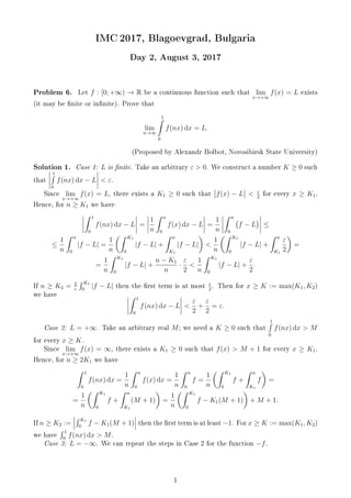
  • 1. IMC 2017, Blagoevgrad, Bulgaria Day 2, August 3, 2017 Problem 6. Let f : [0; +∞) → R be a continuous function such that lim x→+∞ f(x) = L exists (it may be nite or innite). Prove that lim n→∞ 1 0 f(nx) dx = L. (Proposed by Alexandr Bolbot, Novosibirsk State University) Solution 1. Case 1: L is nite. Take an arbitrary ε 0. We construct a number K ≥ 0 such that 1 0 f(nx) dx − L ε. Since lim x→+∞ f(x) = L, there exists a K1 ≥ 0 such that f(x) − L ε 2 for every x ≥ K1. Hence, for n ≥ K1 we have 1 0 f(nx) dx − L = 1 n n 0 f(x) dx − L = 1 n n 0 f − L ≤ ≤ 1 n n 0 |f − L| = 1 n K1 0 |f − L| + n K1 |f − L| 1 n K1 0 |f − L| + n K1 ε 2 = = 1 n K1 0 |f − L| + n − K1 n · ε 2 1 n K1 0 |f − L| + ε 2 . If n ≥ K2 = 2 ε K1 0 |f − L| then the rst term is at most ε 2 . Then for x ≥ K := max(K1, K2) we have 1 0 f(nx) dx − L ε 2 + ε 2 = ε. Case 2: L = +∞. Take an arbitrary real M; we need a K ≥ 0 such that 1 0 f(nx) dx M for every x ≥ K. Since lim x→+∞ f(x) = ∞, there exists a K1 ≥ 0 such that f(x) M + 1 for every x ≥ K1. Hence, for n ≥ 2K1 we have 1 0 f(nx) dx = 1 n n 0 f(x) dx = 1 n n 0 f = 1 n K1 0 f + n K1 f = = 1 n K1 0 f + n K1 (M + 1) = 1 n K1 0 f − K1(M + 1) + M + 1. If n ≥ K2 := K1 0 f − K1(M + 1) then the rst term is at least −1. For x ≥ K := max(K1, K2) we have 1 0 f(nx) dx M. Case 3: L = −∞. We can repeat the steps in Case 2 for the function −f. 1
  • 2. Solution 2. Let F(x) = x 0 f. For t 0 we have 1 0 f(tx) dx = F(t) t . Since lim t→∞ t = ∞ in the denominator and lim t→∞ F (t) = lim t→∞ f(t) = L, L'Hospital's rule proves lim t→∞ F(t) t = lim t→∞ F (t) 1 = lim t→∞ f(t) 1 = L. Then it follows that lim F(n) n = L. Problem 7. Let p(x) be a nonconstant polynomial with real coecients. For every positive integer n, let qn(x) = (x + 1)n p(x) + xn p(x + 1). Prove that there are only nitely many numbers n such that all roots of qn(x) are real. (Proposed by Alexandr Bolbot, Novosibirsk State University) Solution. Lemma. If f(x) = amxm + . . . + a1x + a0 is a polynomial with am = 0, and all roots of f are real, then a2 m−1 − 2amam−2 ≥ 0. Proof. Let the roots of f be w1, . . . , wn. By the Viéte-formulas, m i=1 wi = − am−1 am , ij wiwj = am−2 am , 0 ≤ m i=1 w2 i = m i=1 wi 2 − 2 ij wiwj = am−1 am 2 − 2 am−2 am = a2 m−1 − 2amam−2 a2 m . In view of the Lemma we focus on the asymptotic behavior of the three terms in qn(x) with the highest degrees. Let p(x) = axk + bxk−1 + cxk−2 + . . . and qn(x) = Anxn+k + Bnxn+k−1 + Cnxn+k−2 + . . . ; then qn(x) = (x + 1)n p(x) + xn p(x + 1) = = xn + nxn−1 + n(n − 1) 2 xn−2 + . . . (axk + bxk−1 + cxk−2 + . . .) + xn a xk + kxk−1 + k(k − 1) 2 xk−2 + . . . + b xk−1 + (k − 1)xk−2 + . . . + c xk−2 . . . + . . . = 2a · xn+k + (n + k)a + 2b xn+k−1 + n(n − 1) + k(k − 1) 2 a + (n + k − 1)b + 2c xn+k−2 + . . . , so An = 2a, Bn = (n + k)a + 2b = Cn = n(n − 1) + k(k − 1) 2 a + (n + k − 1)b + 2c. If n → ∞ then B2 n − 2AnCn = na + O(1) 2 − 2 · 2a n2 a 2 + O(n) = −an2 + O(n) → −∞, so B2 n − 2AnCn is eventually negative, indicating that qn cannot have only real roots. 2
  • 3. Problem 8. Dene the sequence A1, A2, . . . of matrices by the following recurrence: A1 = 0 1 1 0 , An+1 = An I2n I2n An (n = 1, 2, . . .) where Im is the m × m identity matrix. Prove that An has n + 1 distinct integer eigenvalues λ0 λ1 . . . λn with multiplicities n 0 , n 1 , . . . , n n , respectively. (Proposed by Snjeºana Majstorovi¢, University of J. J. Strossmayer in Osijek, Croatia) Solution. For each n ∈ N, matrix An is symmetric 2n × 2n matrix with elements from the set {0, 1}, so that all elements on the main diagonal are equal to zero. We can write An = I2n−1 ⊗ A1 + An−1 ⊗ I2, (1) where ⊗ is binary operation over the space of matrices, dened for arbitrary B ∈ Rn×p and C ∈ Rm×s as B ⊗ C :=      b11C b12C . . . b1pC b21C b22C . . . b2pC ... bn1C b12C . . . bnpC      nm×ps . Lemma 1. If B ∈ Rn×n has eigenvalues λi, i = 1, . . . , n and C ∈ Rm×m has eigenvalues µj, j = 1, . . . , m, then B ⊗ C has eigenvalues λiµj, i = 1, . . . , n, j = 1, . . . , m. If B and C are diagonalizable, then A ⊗ B has eigenvectors yi ⊗ zj, with (λi, yi) and (µj, zj) being eigenpairs of B and C, respectively. Proof 1. Let (λ, y) be an eigenpair of B and (µ, z) an eigenpar of C. Then (B ⊗ C)(y ⊗ z) = By ⊗ Cz = λy ⊗ µz = λµ(y ⊗ z). If we take (λ, y) to be an eigenpair of A1 and (µ, z) to be an eigenpair of An−1, then from (1) and Lemma 1 we get An(z ⊗ y) = (I2n−1 ⊗ A1 + An−1 ⊗ I2)(z ⊗ y) = (I2n−1 ⊗ A1)(z ⊗ y) + (An−1 ⊗ I2)(z ⊗ y) = (λ + µ)(z ⊗ y). So the entire spectrum of An can be obtained from eigenvalues of An−1 and A1: just sum up each eigenvalue of An−1 with each eigenvalue of A1. Since the spectrum of A1 is σ(A1) = {−1, 1}, we get σ(A2) = {−1 + (−1), −1 + 1, 1 + (−1), 1 + 1} = {−2, 0(2) , 2} σ(A3) = {−1 + (−2), −1 + 0, −1 + 0, −1 + 2, 1 + (−2), 1 + 0, 1 + 0, 1 + 2} = {−3, (−1)(3) , 1(3) , 3} σ(A4) = {−1 + (−3), −1 + (−1(3) ), −1 + 1(3) , −1 + 3, 1 + (−3), 1 + (−1(3) ), 1 + 1(3) , 1 + 3} = {−4, (−2)(4) , 0(3) , 2(4) , 4}. Inductively, An has n + 1 distinct integer eigenvalues −n, −n + 2, −n + 4, . . . , n − 4, n − 2, n with multiplicities n 0 , n 1 , n 2 , . . . , n n , respectively. Problem 9. Dene the sequence f1, f2, . . . : [0, 1) → R of continuously dierentiable functions by the following recurrence: f1 = 1; fn+1 = fnfn+1 on (0, 1), and fn+1(0) = 1. Show that lim n→∞ fn(x) exists for every x ∈ [0, 1) and determine the limit function. 3
  • 4. (Proposed by Tomá² Bárta, Charles University, Prague) Solution. First of all, the sequence fn is well dened and it holds that fn+1(x) = e x 0 fn(t)dt . (2) The mapping Φ : C([0, 1)) → C([0, 1)) given by Φ(g)(x) = e x 0 g(t)dt is monotone, i.e. if f g on (0, 1) then Φ(f)(x) = e x 0 f(t)dt e x 0 g(t)dt = Φ(g)(x) on (0, 1). Since f2(x) = e x 0 1mathrmdt = ex 1 = f1(x) on (0, 1), we have by induction fn+1(x) fn(x) for all x ∈ (0, 1), n ∈ N. Moreover, function f(x) = 1 1−x is the unique solution to f = f2 , f(0) = 1, i.e. it is the unique xed point of Φ in {ϕ ∈ C([0, 1)) : ϕ(0) = 1}. Since f1 f on (0, 1), by induction we have fn+1 = Φ(fn) Φ(f) = f for all n ∈ N. Hence, for every x ∈ (0, 1) the sequence fn(x) is increasing and bounded, so a nite limit exists. Let us denote the limit g(x). We show that g(x) = f(x) = 1 1−x . Obviously, g(0) = lim fn(0) = 1. By f1 ≡ 1 and (2), we have fn 0 on [0, 1) for each n ∈ N, and therefore (by (2) again) the function fn+1 is increasing. Since fn, fn+1 are positive and increasing also fn+1 is increasing (due to fn+1 = fnfn+1), hence fn+1 is convex. A pointwise limit of a sequence of convex functions is convex, since we pass to a limit n → ∞ in fn(λx + (1 − λ)y) ≤ λfn(x) + (1 − λ)fn(y) and obtain g(λx + (1 − λ)y) ≤ λg(x) + (1 − λ)g(y) for any xed x, y ∈ [0, 1) and λ ∈ (0, 1). Hence, g is convex, and therefore continuous on (0, 1). Moreover, g is continuous in 0, since 1 ≡ f1 ≤ g ≤ f and limx→0+ f(x) = 1. By Dini's Theorem, convergence fn → g is uniform on [0, 1 − ε] for each ε ∈ (0, 1) (a monotone sequence converging to a continuous function on a compact interval). We show that Φ is continuous and therefore fn have to converge to a xed point of Φ. In fact, let us work on the space C([0, 1 − ε]) with any xed ε ∈ (0, 1), · being the supremum norm on [0, 1 − ε]. Then for a xed function h and ϕ − h δ we have sup x∈[0,1−ε] |Φ(h)(x) − Φ(ϕ)(x)| = sup x∈[0,1−ε] e x 0 h(t)dt 1 − e x 0 ϕ(t)−h(t)dt ≤ C(eδ − 1) 2Cδ for δ 0 small enough. Hence, Φ is continuous on C([0, 1−ε]). Let us assume for contradiction that Φ(g) = g. Hence, there exists η 0 and x0 ∈ [0, 1 − ε] such that |Φ(g)(x0) − g(x0)| η. There exists δ 0 such that Φ(ϕ) − Φ(g) 1 3 η whenever ϕ − g δ. Take n0 so large that fn − g min{δ, 1 3 η} for all n ≥ n0. Hence, fn+1 − Φ(g) = Φ(fn) − Φ(g) 1 3 η. On the other hand, we have |fn+1(x0)−Φ(g)(x0)| |Φ(g)(x0)−g(x0)|−|g(x0)−fn+1(x0)| η−1 3 η = 2 3 η, contradiction. So, Φ(g) = g. Since f is the only xed point of Φ in {ϕ ∈ C([0, 1 − ε]) : ϕ(0) = 1}, we have g = f on [0, 1 − ε]. Since ε ∈ (0, 1) was arbitrary, we have limn→∞ fn(x) = 1 1−x for all x ∈ [0, 1). 4
  • 5. Problem 10. Let K be an equilateral triangle in the plane. Prove that for every p 0 there exists an ε 0 with the following property: If n is a positive integer, and T1, . . . , Tn are non-overlapping triangles inside K such that each of them is homothetic to K with a negative ratio, and n =1 area(T ) area(K) − ε, then n =1 perimeter(T ) p. (Proposed by Fedor Malyshev, Steklov Math. Inst. and Ilya Bogdanov, MIPT, Moscow) Solution. For an arbitrary ε 0 we will establish a lower bound for the sum of perimeters that would tend to +∞ as ε → +0; this solves the problem. Rotate and scale the picture so that one of the sides of K is the segment from (0, 0) to (0, 1), and stretch the picture horizontally in such a way that the projection of K to the x axis is [0, 1]. Evidently, we may work with the lengths of the projections to the x or y axis instead of the perimeters and consider their sum, that is why we may make any ane transformation. Let fi(a) be the length of intersection of the straight line {x = a} with Ti and put f(a) = i fi(a). Then f is piece-wise increasing with possible downward gaps, f(a) ≤ 1 − a, and 1 0 f(x) dx ≥ 1 2 − ε. Let d1, . . . , dN be the values of the gaps of f. Every gap is a sum of side-lengths of some of Ti and every Ti contributes to one of dj, we therefore estimate the sum of the gaps of f. In the points of dierentiability of f we have f (a) ≥ f(a)/a; this follows from fi(a) ≥ fi(a)/a after summation. Indeed, if fi is zero this inequality holds trivially, and if not then fi = 1 and the inequality reads fi(a) ≤ a, which is clear from the denition. Choose an integer m = 1/(8ε) (considering ε suciently small). Then for all k = 0, 1, . . . , [(m − 1)/2] in the section of K by the strip k/m ≤ x ≤ (k + 1)/m the area, cov- ered by the small triangles Ti is no smaller than 1/(2m) − ε ≥ 1/(4m). Thus (k+1)/m k/m f (x) dx ≥ (k+1)/m k/m f(x) dx x ≥ m k + 1 (k+1)/m k/m f(x) dx ≥ m k + 1 · 1 4m = 1 4(k + 1) . Hence, 1/2 0 f (x) dx ≥ 1 4 1 1 + · · · + 1 [(m − 1)/2] . The right hand side tends to innity as ε → +0. On the other hand, the left hand side equals f(1/2) + xi1/2 di; hence i di also tends to innity. 5