1. Proceedings of the Institute of Acoustics & Belgium Acoustical Society
Noise in the Built Environment, Ghent, 29-30 April 2010
Vol. 32. Pt 3. 2010
COMBINED ASSESSMENT OF NOISE AND
AIR POLLUTION CAUSED BY ROAD TRAFFIC
B De Coensel Ghent University, Department of Information Technology, Ghent, Belgium
A Can Ghent University, Department of Information Technology, Ghent, Belgium
M Madireddy VITO, Transport and Mobility, Mol, Belgium, and Ghent University
I De Vlieger VITO, Transport and Mobility, Mol, Belgium
D Botteldooren Ghent University, Department of Information Technology, Ghent, Belgium
Abstract
Road traffic is a major source of noise and air pollution in the urban environment. Hence, traffic
management solutions are increasingly called for to address problems of noise and atmospheric
pollution. Because changes in traffic flow do not necessarily influence transport mobility, noise and
air quality in the same way, there is a clear need for a combined approach. This paper reports on
the construction of a model which combines microscopic traffic simulation with emission submodels
for noise and air pollutants, and its application to a case study area. The approach presented could
be of inspiration for the construction of guidance tools for urban planning practice.
1 INTRODUCTION
Traffic congestion causes travel delays, and thus imposes a substantial cost on society. Urban
traffic management solutions, such as introducing variable speed limits, installing express lanes or
optimizing traffic signal timing, are commonly used to moderate congestion in urban areas, where
expanding the road network is not feasible. Although the potential of traffic management to reduce
travel delays is widely accepted, the side-effects on noise and air quality are much less clear.
Improving traffic conditions does not necessarily mean that there is less noise or air pollutant
emission. Most studies on the influence of traffic management measures on emission consider air
pollution and noise emissions at a single intersection at most1,2
. On the one hand, field experiments
during which emissions are measured are quite complex to carry out. On the other hand,
computational models for estimating emissions that return realistic results for the stop-and-go
behavior of vehicles in urban environment have not been available until recently.
Small-scale changes in infrastructure can have a large influence on traffic flows; an example is the
installment of green waves, i.e. synchronization of traffic lights at several consecutive signalized
intersections. In order to study the impact of such measures on traffic flow, researchers are more
and more considering the use of microscopic traffic simulation models. Coupled with models for
instantaneous vehicle emissions, this approach offers great potential to study the influence of traffic
management measures on traffic flow, noise and air pollutant emission simultaneously. In this
paper, such a combined model is presented, and results for a case study are discussed.
2 GENERAL METHODOLOGY
2.1 Microscopic traffic simulation
Microscopic traffic simulation models consider the behavior of individual vehicles, as compared to
macroscopic models that only consider the traffic flow as a whole. Behavioral rules, such as when
to change lanes, when to overtake or how much distance to keep to the vehicle in front, form the
core of most microsimulation models. They require much more effort to construct, as compared to

2. Proceedings of the Institute of Acoustics & Belgium Acoustical Society
Noise in the Built Environment, Ghent, 29-30 April 2010
Vol. 32. Part 3. 2010
macroscopic models, because the (urban) environment has to be modelled in great detail (locations
of kerbs and stop lines, exact size of intersections etc.). Therefore, they are only useful to study
small to medium sized areas (e.g. part of a city). As a benefit, they allow to estimate the impact of
detailed infrastructure changes, because the influence of braking and accelerating is taken into
account. In this work, Paramics3
, a commercially available microsimulation tool, is used as the
modelling software. The output of the model consists of the instantaneous position, speed and
acceleration of each vehicle at each timestep of the simulation (usually 0.5s or less).
2.2 Noise and air pollutant emission
The Harmonoise vehicle noise emission model4
is used in this work to calculate instantaneous
noise emissions. It produces point source sound power levels at a specific height above the ground,
on the basis of vehicle type, speed and acceleration. Two sources of noise are considered: rolling
noise generated by tire-road interaction, and powertrain and exhaust noise. Emissions are
calculated on a 1/3-octave band basis; however, in this work we will only consider the total (A-
weighted) source sound power level, noted as LW. When the noise emission of a vehicle trip through
the network is considered, we define LW
avg
as the average source sound power level of the
particular vehicle over the course of its trip (energetically averaged). In a similar way, the total
source sound power level LW
tot
for the trip of a single vehicle can be defined, which also takes into
account the duration of the trip. The Harmonoise model was specifically developed with microscopic
traffic simulation models in mind, and has been validated widely on an European scale, using a
large number of vehicles, driven on a wide scale of road surface types. The vehicle classes defined
in the Harmonoise model represent the average noise emission of the European vehicle fleet.
The VERSIT+ vehicle exhaust emission model5,6
is used in this work to calculate instantaneous
CO2, NOx and PM10 emissions. This model, developed and supported by TNO, is based on more
than 12500 measurements on vehicles of a wide range of categories and makes. It takes into
account detailed effects such as cold started engines or the wearing of tires and brakes. A derived
model (VERSIT+micro) was recently developed by TNO, specifically targeted at a coupling with
microscopic traffic simulation models. For this, emission parameters of different vehicles (with
varying fuel type) were aggregated into a prototypical vehicle emission model representing the
average emission of the Dutch vehicle fleet. Only two main classes of vehicles are considered: light
duty (including passenger cars) and heavy duty vehicles. As with the Harmonoise emission model,
instantaneous emissions are calculated on the basis of vehicle type (light or heavy), speed and
acceleration, extracted from the microscopic traffic simulation model.
It has to be noted that only emissions are considered in this paper; the propagation of sound and
the dispersion of air pollutants are not modelled.
3 CASE STUDY
3.1 Construction of the microsimulation network
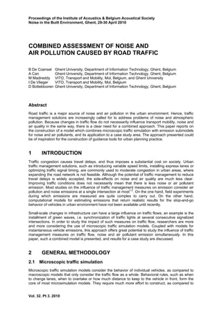
To illustrate the above methodology, the case study area “Zurenborg” was selected. The area is
located in the southeastern part of the 19th century city belt of Antwerp, Belgium. Figure 1, left,
shows a map of the region. The area is bounded by a freeway and a major road in the east, a major
arterial road in the north and a railway track along the southwest. The major arterial road (the
“Plantin en Moretuslei”) connects the city of Antwerp (situated at the west side of the area) with
suburban areas in the east. This road has 2 lanes in each direction, and implements traffic signal
synchronization. More in particular, during morning rush hour, all signals along this road operate at
the same cycle time (60s to 90s, depending on the presence of pedestrians or buses), and the
temporal offset of the cylce of each intersection is set up such that vehicles travelling from east to
west encounter only green lights, when driving at the desired speed of 50 km/h. A similar signal
setting is applied in the reverse direction during the evening rush hour.

3. Proceedings of the Institute of Acoustics & Belgium Acoustical Society
Noise in the Built Environment, Ghent, 29-30 April 2010
Vol. 32. Part 3. 2010
A microsimulation network (Figure 1, right) was constructed on the basis of GIS data (roads,
buildings, and aerial photographs) and traffic light timing data (from the Antwerp police department).
Network wide traffic demands were calibrated for the morning rush-hour, based on traffic counts
made available by the Flemish Dept. of Mobility and Public Works. Two types of vehicles (light and
heavy duty) are considered, which are linked to the respective emission classes of the Harmonoise
and VERSIT+ emission models. A railway track passes through the area, but this is not modelled. In
order to show how this model can be used to investigate the influence of traffic management
measures, three different scenarios are considered. The first scenario represents the current
situation, with a green wave along the arterial road. The second scenario is identical to the first one,
except for the traffic lights along the arterial road, which are not synchronized. This allows us to see
the influence of the installment of the green wave on emissions. In order to desynchronize the
signals, a small but random number of seconds was added to or subtracted from the cycle times.
This way, a wide range of waiting times at each intersection is encountered over the course of the
simulation run. In the third scenario, speed limits have been reduced as compared to the first
scenario, from 50 km/h to 30 km/h along the arterial road. The signalized intersection offsets have
been adjusted to this new desired speed, so there is still a green wave in this scenario.
Figure 1 – (left) Map of the case study area; (right) screenshot of the
microsimulation network, with signalized intersections circled in red.
The microscopic traffic simulation time considered is 1 hour, with a simulation timestep of 0.5s.
Vehicles are loaded onto the network at the edge roads along the sides of the network, according to
the traffic demands (which are the same for all scenarios). The traffic intensity along the major
arterial road during rush hour, from east to west, is between 700 and 1000 vehicles/hour, depending
on the segment that is considered (vehicles also enter along the side streets). During simulation,
locations and kinematic properties of all vehicles are recorded at each time step, for subsequent
calculation of emissions.
3.2 Individual trip emissions
In this section, we will consider the total emission of vehicles during their trip through the network
(simply called the trip emission). Because the northern arterial road is of main focus, only the
emissions of the vehicles driving along this road, from east to west into the city, are considered for
the analysis in this section. Table 1 gives an overview of the average trip emissions. Comparable
trends are found for both light and heavy duty vehicles. It should be mentioned that the optimal

4. Proceedings of the Institute of Acoustics & Belgium Acoustical Society
Noise in the Built Environment, Ghent, 29-30 April 2010
Vol. 32. Part 3. 2010
conditions could be different when the cross-flow direction is also taken into account, although this
direction carries much less traffic (200 to 300 vehicles/hour).
Considering noise, it can be seen that the average vehicle sound power would decrease by 0.6 (for
heavy duty vehicles) to 0.9 dB(A) (for light duty vehicles) when the green wave is removed.
However, because trips would take longer to complete, the average total emission would still
increase with 0.1 to 0.3 dB(A). The effect of the green wave on total noise emissions thus seems to
be negligible. On the other hand, reducing speeds has a clear beneficial influence on noise, with
reductions in total emission from 1.2 to 1.9 dB(A).
Considering air pollutant emissions, it can be seen that removing the green wave would increase
emissions by 10 to 13%, for all types of pollutants. When speeds are lowered to 30 km/h, the
picture is not that clear anymore: CO2 and NOx emissions would drop, but PM10 emissions would
rise by 11% to 19%. The slower speeds in scenario 3 cause the vehicles to consume less fuel and,
as a consequence, to emit less pollutants per second on average, but vehicles also take more time
to complete their trip. For CO2 and NOx emissions, the longer trip duration is overcompensated by
the reduction in emissions per second, while this is not the case for PM10.
Figure 2 shows the histograms of the trip emissions for light duty vehicles travelling along the main
arterial road. Overall, the most compact distributions are found for scenario 3, which indicates that
the flow is most homogenous with the lower speed limit of 30 km/h.
Table 1 – Average trip durations and total trip emissions for the different scenarios.
Scenario 1 Scenario 2 Scenario 3
Speed limit
Green wave?
Avg. trip duration
50 km/h
Yes
217s
50 km/h
No
274s (+26%)
30 km/h
Yes
311s (+43%)
Light duty vehicles
LW
avg
LW
tot
CO2
NOx
PM10
93.9 dBA
117.2 dBA
1329 g
3.355 g
0.2236 g
93.0 dBA (-0.9)
117.3 dBA (+0.1)
1502 g (+13%)
3.748 g (+12%)
0.2495 g (+12%)
90.4 dBA (-3.5)
115.3 dBA (-1.9)
1081 g (-19%)
2.188 g (-35%)
0.2479 g (+11%)
Heavy duty vehicles
LW
avg
LW
tot
CO2
NOx
PM10
106.8 dBA
130.6 dBA
5804 g
50.94 g
2.0326 g
106.2 dBA (-0.6)
130.9 dBA (+0.3)
6402 g (+10%)
56.15 g (+10%)
2.2846 g (+12%)
104.4 dBA (-2.4)
129.4 dBA (-1.2)
4450 g (-23%)
39.52 g (-22%)
2.4142 g (+19%)
3.3 Spatial distribution of emissions
In this section, we will consider the spatial distribution of noise and air pollutant emission. A
rectangular subregion with a size of 1400m by 350m, surrounding the northern arterial road, was
selected. Note that all vehicles are considered in this section, not only those that drive along the
arterial road from east to west. Figure 3 shows the spatial emission distributions for the first
scenario, and the differences between the other scenarios and the first scenario. For the noise
maps, hourly equivalent source power levels are aggregated to a grid of emission points, with a
spatial resolution of 5m. For the air pollutant emission maps, total emissions are aggregated into
bins with a surface of 25 m2
.
Removal of the green wave, or reduction of the limit speed, causes changes in noise emission that
are more or less evenly distributed along the arterial road. In contrast, changes in air pollutant

5. Proceedings of the Institute of Acoustics & Belgium Acoustical Society
Noise in the Built Environment, Ghent, 29-30 April 2010
Vol. 32. Part 3. 2010
emission are more concentrated, because of the greater influence of acceleration on air pollutant
emission. Removal of the green wave would result in much higher emissions (up to 50% locally)
near the downstream arms of the intersections, where vehicles accelerate. In contrast, a speed
reduction would have the highest impact in the stretches of road in between intersections.
Figure 2 – Histograms of trip emissions for the three scenarios.
Figure 3 – Spatial ditributions of emissions along the arterial road (bins of 25m2
).

6. Proceedings of the Institute of Acoustics & Belgium Acoustical Society
Noise in the Built Environment, Ghent, 29-30 April 2010
Vol. 32. Part 3. 2010
4 CONCLUSIONS
In this paper, a computational approach for assessing the environmental impact of traffic
management measures was described, which combines microscopic traffic simulation with emission
models for noise and air pollutants. Simulation results for a case study area were presented,
including scenarios with a green wave and a speed reduction. It was found that changes in traffic
flow do not always influence travel times, noise and air pollutant emission (CO2, NOx and PM10) in
the same way. The results indicate the importance of a combined approach, when considering the
environmental impact of urban traffic management decisions.
ACKNOWLEDGMENTS
This project was partly funded by the Flemish Policy Research Centre for Mobility & Public Works
(Steunpunt Mobiliteit en Openbare Werken, spoor Verkeersveiligheid). Bert De Coensel is a
postdoctoral fellow, and Arnaud Can is a visiting postdoctoral fellow of the Research Foundation–
Flanders (FWO–Vlaanderen); the support of this organisation is also gratefully acknowledged.
REFERENCES
1. S. Pandian, S. Gokhale and A. K. Ghoshal, “Evaluating effects of traffic and vehicle
characteristics on vehicular emissions near traffic intersections”, Transportation Research
Part D 14(3):180-196, 2009.
2. B. De Coensel, D. Botteldooren, F. Vanhove and S. Logghe, “Microsimulation based
corrections on the road traffic noise emission near intersections”, Acta Acustica united with
Acustica 93(2):241-252, 2007.
3. Paramics is developed by Quadstone (http://www.paramics-online.com/).
4. H. Jonasson, U. Sandberg, G. van Blokland, J. Ejsmont, G. Watts and M. Luminari, “Source
modelling of road vehicles”, Technical Report HAR11TR-041210-SP10, Deliverable 9 of the
Harmonoise project, 2004.
5. R. Smit, R. Smokers and E. Rabé, “A new modelling approach for road traffic emissions:
VERSIT+”, Transportation Research Part D 12(6):414-422, 2007.
6. N. E. Ligterink and R. De Lange, “Refined vehicle and driving-behaviour dependencies in
the VERSIT+ emission model”, In Proceedings of the Joint 17th Transport and Air Pollution
Symposium and 3rd Environment and Transport Symposium (ETTAP), Toulouse, France,
June 2009.