Machine learning

1. Machine Learning
Basic Concepts
Feature'2
'
Feature'1'
!"#$%&"'(
'
!"#$%&"')'
*"+,-,./'0.%/1#&2'

2. Terminology
Machine Learning, Data Science, Data Mining, Data Analysis, Sta-
tistical Learning, Knowledge Discovery in Databases, Pattern Dis-
covery.

3. Data everywhere!
1. Google: processes 24 peta bytes of data per day.
2. Facebook: 10 million photos uploaded every hour.
3. Youtube: 1 hour of video uploaded every second.
4. Twitter: 400 million tweets per day.
5. Astronomy: Satellite data is in hundreds of PB.
6. . . .
7. “By 2020 the digital universe will reach 44
zettabytes...”
The Digital Universe of Opportunities: Rich Data and the
Increasing Value of the Internet of Things, April 2014.
That’s 44 trillion gigabytes!

4. Data types
Data comes in different sizes and also flavors (types):
Texts
Numbers
Clickstreams
Graphs
Tables
Images
Transactions
Videos
Some or all of the above!

5. Smile, we are ’DATAFIED’ !
• Wherever we go, we are “datafied”.
• Smartphones are tracking our locations.
• We leave a data trail in our web browsing.
• Interaction in social networks.
• Privacy is an important issue in Data Science.

6. The Data Science process
T
i
m
e
DATA COLLECTION
Static
Data.
Domain
expertise
1 3
4
5
!
DB%
DB
EDA
MACHINE LEARNING
Visualization
Descriptive
statistics,
Clustering
Research
questions?
Classification,
scoring, predictive
models,
clustering, density
estimation, etc.
Data-driven
decisions
Application
deployment
Model%(f)%
Yes!/!
90%!
Predicted%class/risk%
A!and!B!!!C!
Dashboard
Static
Data.
2 DATA PREPARATION
Data!cleaning!
+
+
+
+
+
-
+
+
-
-
-
-
-
-
+
Feature/variable!
engineering!

7. Applications of ML
• We all use it on a daily basis. Examples:

8. Machine Learning
• Spam filtering
• Credit card fraud detection
• Digit recognition on checks, zip codes
• Detecting faces in images
• MRI image analysis
• Recommendation system
• Search engines
• Handwriting recognition
• Scene classification
• etc...

9. Interdisciplinary field
ML!
Statistics!
Visualization!
Economics!
Databases!
Signal
processing!
Engineering !
Biology!

10. ML versus Statistics
Statistics:
• Hypothesis testing
• Experimental design
• Anova
• Linear regression
• Logistic regression
• GLM
• PCA
Machine Learning:
• Decision trees
• Rule induction
• Neural Networks
• SVMs
• Clustering method
• Association rules
• Feature selection
• Visualization
• Graphical models
• Genetic algorithm
http://statweb.stanford.edu/~jhf/ftp/dm-stat.pdf

11. Machine Learning definition
“How do we create computer programs that improve with experi-
ence?”
Tom Mitchell
http://videolectures.net/mlas06_mitchell_itm/

12. Machine Learning definition
“How do we create computer programs that improve with experi-
ence?”
Tom Mitchell
http://videolectures.net/mlas06_mitchell_itm/
“A computer program is said to learn from experience E with
respect to some class of tasks T and performance measure P, if
its performance at tasks in T, as measured by P, improves with
experience E. ”
Tom Mitchell. Machine Learning 1997.

13. Supervised vs. Unsupervised
Given: Training data: (x1, y1), . . . , (xn, yn) / xi ∈ Rd and yi is the
label.
example x1 → x11 x12 . . . x1d y1 ← label
. . . . . . . . . . . . . . . . . .
example xi → xi1 xi2 . . . xid yi ← label
. . . . . . . . . . . . . . . . . .
example xn → xn1 xn2 . . . xnd yn ← label

14. Supervised vs. Unsupervised
Given: Training data: (x1, y1), . . . , (xn, yn) / xi ∈ Rd and yi is the
label.
example x1 → x11 x12 . . . x1d y1 ← label
. . . . . . . . . . . . . . . . . .
example xi → xi1 xi2 . . . xid yi ← label
. . . . . . . . . . . . . . . . . .
example xn → xn1 xn2 . . . xnd yn ← label

15. Supervised vs. Unsupervised
Unsupervised learning:
Learning a model from unlabeled data.
Supervised learning:
Learning a model from labeled data.

16. Unsupervised Learning
Training data:“examples” x.
x1, . . . , xn, xi ∈ X ⊂ Rn
• Clustering/segmentation:
f : Rd −→ {C1, . . . Ck} (set of clusters).
Example: Find clusters in the population, fruits, species.

17. Unsupervised learning
Feature'2
'
Feature'1'

18. Unsupervised learning
Feature'2
'
Feature'1'

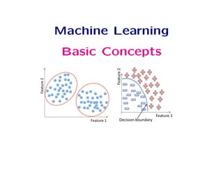
19. Unsupervised learning
Feature'2
'
Feature'1'
Methods: K-means, gaussian mixtures, hierarchical clustering,
spectral clustering, etc.

20. Supervised learning
Training data:“examples” x with “labels” y.
(x1, y1), . . . , (xn, yn) / xi ∈ Rd
• Classification: y is discrete. To simplify, y ∈ {−1, +1}
f : Rd −→ {−1, +1} f is called a binary classifier.
Example: Approve credit yes/no, spam/ham, banana/orange.

21. Supervised learning
!#$%'(
'
!#$%')'

22. Supervised learning
!#$%'(
'
!#$%')'
*+,-,./'0.%/1#2'

23. Supervised learning
!#$%'(
'
!#$%')'
*+,-,./'0.%/1#2'
Methods: Support Vector Machines, neural networks, decision
trees, K-nearest neighbors, naive Bayes, etc.

24. Supervised learning
Classification:
!#$%'(
'
!#$%')'
!#$%'(
'
!#$%')'
!#$%'('
!#$%')'
!#$%'('
!#$%')'
!#$%'(
'
!#$%')'

25. Supervised learning
Non linear classification

26. Supervised learning
Training data:“examples” x with “labels” y.
(x1, y1), . . . , (xn, yn) / xi ∈ Rd
• Regression: y is a real value, y ∈ R
f : Rd −→ R f is called a regressor.
Example: amount of credit, weight of fruit.

27. Supervised learning
Regression:
!
#$%'($)
Example: Income in function of age, weight of the fruit in function
of its length.

28. Supervised learning
Regression:
!
#$%'($)

29. Supervised learning
Regression:
!
#$%'($)

30. Supervised learning
Regression:
!
#$%'($)

31. Training and Testing
!#$%$%'()*'
+,'-./$*01'
+/2).'345'

32. Training and Testing
!#$%$%'()*'
+,'-./$*01'
+/2).'345'
6%7/1)8''
)%2)8''
#)8''
4#1$.9'(*#*:(8'
;$7/2)'
=)2$*'#1/:%*''
=)2$*'9)(?%/'

33. K-nearest neighbors
• Not every ML method builds a model!
• Our first ML method: KNN.
• Main idea: Uses the similarity between examples.
• Assumption: Two similar examples should have same labels.
• Assumes all examples (instances) are points in the d dimen-
sional space Rd.

34. K-nearest neighbors
• KNN uses the standard Euclidian distance to define nearest
neighbors.
Given two examples xi and xj:
d(xi, xj) =
v
u
u
u
t
d
X
k=1
(xik − xjk)2

35. K-nearest neighbors
Training algorithm:
Add each training example (x, y) to the dataset D.
x ∈ Rd, y ∈ {+1, −1}.

36. K-nearest neighbors
Training algorithm:
Add each training example (x, y) to the dataset D.
x ∈ Rd, y ∈ {+1, −1}.
Classification algorithm:
Given an example xq to be classified. Suppose Nk(xq) is the set of
the K-nearest neighbors of xq.
ŷq = sign(
X
xi∈Nk(xq)
yi)

37. K-nearest neighbors
3-NN. Credit: Introduction to Statistical Learning.

38. K-nearest neighbors
3-NN. Credit: Introduction to Statistical Learning.
Question: Draw an approximate decision boundary for K = 3?

39. K-nearest neighbors
Credit: Introduction to Statistical Learning.

40. K-nearest neighbors
Question: What are the pros and cons of K-NN?

41. K-nearest neighbors
Question: What are the pros and cons of K-NN?
Pros:
+ Simple to implement.
+ Works well in practice.
+ Does not require to build a model, make assumptions, tune
parameters.
+ Can be extended easily with news examples.

42. K-nearest neighbors
Question: What are the pros and cons of K-NN?
Pros:
+ Simple to implement.
+ Works well in practice.
+ Does not require to build a model, make assumptions, tune
parameters.
+ Can be extended easily with news examples.
Cons:
- Requires large space to store the entire training dataset.
- Slow! Given n examples and d features. The method takes
O(n × d) to run.
- Suffers from the curse of dimensionality.

43. Applications of K-NN
1. Information retrieval.
2. Handwritten character classification using nearest neighbor in
large databases.
3. Recommender systems (user like you may like similar movies).
4. Breast cancer diagnosis.
5. Medical data mining (similar patient symptoms).
6. Pattern recognition in general.

44. Training and Testing
!#$%$%'()*'
+,'-./$*01'
+/2).'345'
6%7/1)8''
)%2)8''
#)8''
4#1$.9'(*#*:(8'
;$7/2)'
=)2$*'#1/:%*''
=)2$*'9)(?%/'
Question: How can we be confident about f?

45. Training and Testing
• We calculate Etrain the in-sample error (training error or em-
pirical error/risk).
Etrain(f) =
n
X
i=1
`oss(yi, f(xi))

46. Training and Testing
• We calculate Etrain the in-sample error (training error or em-
pirical error/risk).
Etrain(f) =
n
X
i=1
`oss(yi, f(xi))
• Examples of loss functions:
– Classification error:
`oss(yi, f(xi)) =
(
1 if sign(yi) 6= sign(f(xi))
0 otherwise

47. Training and Testing
• We calculate Etrain the in-sample error (training error or em-
pirical error/risk).
Etrain(f) =
n
X
i=1
`oss(yi, f(xi))
• Examples of loss functions:
– Classification error:
`oss(yi, f(xi)) =
(
1 if sign(yi) 6= sign(f(xi))
0 otherwise
– Least square loss:
`oss(yi, f(xi)) = (yi − f(xi))2

48. Training and Testing
• We calculate Etrain the in-sample error (training error or em-
pirical error/risk).
Etrain(f) =
n
X
i=1
`oss(yi, f(xi))
• We aim to have Etrain(f) small, i.e., minimize Etrain(f)

49. Training and Testing
• We calculate Etrain the in-sample error (training error or em-
pirical error/risk).
Etrain(f) =
n
X
i=1
`oss(yi, f(xi))
• We aim to have Etrain(f) small, i.e., minimize Etrain(f)
• We hope that Etest(f), the out-sample error (test/true error),
will be small too.

50. Overfitting/underfitting
An intuitive example

51. Structural Risk Minimization
Predic'on*Error
*
Low*******************************************Complexity*of*the*model*************************************High*
____Test*error****
____Training*error*
High*Bias****** * * * * * * * ***Low*Bias**
Low*Variance* * * * * * * * *High*Variance*
UnderfiAng****************Good*models** * * *OverfiAng * ***********

52. Training and Testing
!#$%'
()'
!#$%'
()'
!#$%'
()'

53. Training and Testing
!#$%'
()'
!#$%'
()'
High bias (underfitting)
!#$%'
()'

54. Training and Testing
!#$%'
()'
!#$%'
()'
High bias (underfitting)
!#$%'
()'
High variance (overfitting)

55. Training and Testing
!#$%'
()'
!#$%'
()'
High bias (underfitting) Just right!
!#$%'
()'
High variance (overfitting)

56. Avoid overfitting
In general, use simple models!
• Reduce the number of features manually or do feature selec-
tion.
• Do a model selection (ML course).
• Use regularization (keep the features but reduce their impor-
tance by setting small parameter values) (ML course).
• Do a cross-validation to estimate the test error.

57. Regularization: Intuition
We want to minimize:
Classification term + C × Regularization term
n
X
i=1
`oss(yi, f(xi)) + C × R(f)

58. Regularization: Intuition
!#$%'
()'
!#$%'
()'
!#$%'
()'
f(x) = λ0 + λ1x ... (1)
f(x) = λ0 + λ1x + λ2x2 ... (2)
f(x) = λ0 + λ1x + λ2x2 + λ3x3 + λ4x4 ... (3)
Hint: Avoid high-degree polynomials.

59. Train, Validation and Test
TRAIN VALIDATION TEST
Example: Split the data randomly into 60% for training, 20% for
validation and 20% for testing.

60. Train, Validation and Test
TRAIN VALIDATION TEST
1. Training set is a set of examples used for learning a model
(e.g., a classification model).

61. Train, Validation and Test
TRAIN VALIDATION TEST
1. Training set is a set of examples used for learning a model
(e.g., a classification model).
2. Validation set is a set of examples that cannot be used for
learning the model but can help tune model parameters (e.g.,
selecting K in K-NN). Validation helps control overfitting.

62. Train, Validation and Test
TRAIN VALIDATION TEST
1. Training set is a set of examples used for learning a model
(e.g., a classification model).
2. Validation set is a set of examples that cannot be used for
learning the model but can help tune model parameters (e.g.,
selecting K in K-NN). Validation helps control overfitting.
3. Test set is used to assess the performance of the final model
and provide an estimation of the test error.

63. Train, Validation and Test
TRAIN VALIDATION TEST
1. Training set is a set of examples used for learning a model
(e.g., a classification model).
2. Validation set is a set of examples that cannot be used for
learning the model but can help tune model parameters (e.g.,
selecting K in K-NN). Validation helps control overfitting.
3. Test set is used to assess the performance of the final model
and provide an estimation of the test error.
Note: Never use the test set in any way to further tune
the parameters or revise the model.

64. K-fold Cross Validation
A method for estimating test error using training data.
Algorithm:
Given a learning algorithm A and a dataset D
Step 1: Randomly partition D into k equal-size subsets D1, . . . , Dk
Step 2:
For j = 1 to k
Train A on all Di, i ∈ 1, . . . k and i 6= j, and get fj.
Apply fj to Dj and compute EDj
Step 3: Average error over all folds.
k
X
j=1
(EDj)

65. Confusion matrix
!#$%$' (')*%$'
!#$%$' !#$%'()*)+$%,!- ./0($%'()*)+$%,.-
(')*%$' ./0($%1$2/*)+$%,.1- !#$%1$2/*)+$%,!1-
344#/45 +,!-.-,(/-0-+,!-.-,(-.-1!-.-1(/
$4)()'6 ,!-0-+,!-.-1!/
7$6()*)+)*5%,8$4/00- ,!-0-+,!-.-1(/
79$4):)4)*5 ,(-0-+,(-.-1!/
34*#/0%;/$0%
$=)4*$=%;/$0
,2'-3'45'6%*)'-7-3#$%$'-34'8$5%$6#-%2*%-*4'-
544'5%
,2'-3'45'6%*)'-7-3#$%$'-5*#'#-%2*%-9'4'-
34'8$5%'8-*#-3#$%$'
,2'-3'45'6%*)'-7-6')*%$'-5*#'#-%2*%-9'4'-
34'8$5%'8-*#-6')*%$'
,2'-3'45'6%*)'-7-34'8$5%$6#-%2*%-*4'-544'5%

66. Evaluation metrics
!#$%$' (')*%$'
!#$%$' !#$%'()*)+$%,!- ./0($%'()*)+$%,.-
(')*%$' ./0($%1$2/*)+$%,.1- !#$%1$2/*)+$%,!1-
344#/45 +,!-.-,(/-0-+,!-.-,(-.-1!-.-1(/
$4)()'6 ,!-0-+,!-.-1!/
7$6()*)+)*5%,8$4/00- ,!-0-+,!-.-1(/
79$4):)4)*5 ,(-0-+,(-.-1!/
34*#/0%;/$0%
$=)4*$=%;/$0
,2'-3'45'6%*)'-7-3#$%$'-34'8$5%$6#-%2*%-*4'-
544'5%
,2'-3'45'6%*)'-7-3#$%$'-5*#'#-%2*%-9'4'-
34'8$5%'8-*#-3#$%$'
,2'-3'45'6%*)'-7-6')*%$'-5*#'#-%2*%-9'4'-
34'8$5%'8-*#-6')*%$'
,2'-3'45'6%*)'-7-34'8$5%$6#-%2*%-*4'-544'5%

67. Terminology review
Review the concepts and terminology:
Instance, example, feature, label, supervised learning, unsu-
pervised learning, classification, regression, clustering, pre-
diction, training set, validation set, test set, K-fold cross val-
idation, classification error, loss function, overfitting, under-
fitting, regularization.

68. Machine Learning Books
1. Tom Mitchell, Machine Learning.
2. Abu-Mostafa, Yaser S. and Magdon-Ismail, Malik and Lin,
Hsuan-Tien, Learning From Data, AMLBook.
3. The elements of statistical learning. Data mining, inference,
and prediction T. Hastie, R. Tibshirani, J. Friedman.
4. Christopher Bishop. Pattern Recognition and Machine Learn-
ing.
5. Richard O. Duda, Peter E. Hart, David G. Stork. Pattern
Classification. Wiley.

69. Machine Learning Resources
• Major journals/conferences: ICML, NIPS, UAI, ECML/PKDD,
JMLR, MLJ, etc.
• Machine learning video lectures:
http://videolectures.net/Top/Computer_Science/Machine_Learning/
• Machine Learning (Theory):
http://hunch.net/
• LinkedIn ML groups: “Big Data” Scientist, etc.
• Women in Machine Learning:
https://groups.google.com/forum/#!forum/women-in-machine-learning
• KDD nuggets http://www.kdnuggets.com/

70. Credit
• The elements of statistical learning. Data mining, inference,
and prediction. 10th Edition 2009. T. Hastie, R. Tibshirani,
J. Friedman.
• Machine Learning 1997. Tom Mitchell.