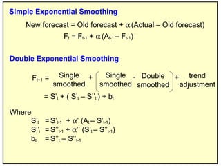
1. Simple Exponential Smoothing New forecast = Old forecast + (Actual – Old forecast) F t = F t-1 + (A t-1 – F t-1 ) Double Exponential Smoothing = S’ t + ( S’ t – S’’ t ) + b t S’ t = S’ t-1 + ’ (A t – S’ t-1 ) S’’ t = S’’ t-1 + ’’ (S’ t – S’’ t-1 ) b t = S’’ t – S’’ t-1 Where F t+1 = Single smoothed Single smoothed Double smoothed trend adjustment + + -
2. Linear trend Y t = + t n ty - t y = n t 2 - ( t) 2 y - t n n t t 2 1 1 1 2 3 5 3 6 14 4 10 30 5 15 55 6 21 91 7 28 140 8 36 204 9 45 285 10 55 385 11 66 506 12 78 650 13 91 819 14 105 1,015 15 120 1,240 16 136 1,496 17 153 1,785 18 171 2,109 19 190 2,470 20 210 2,870
3. Parabolic trend Y t = + t + t 2 with t=0 at the center of the data ty = t 2 y - t 2 n = n t 4 - ( t 2 ) 2 n t 2 y - t 2 y
4. Simple linear regression Y = a + bx a y - x n b = n ( x 2 ) - ( x) 2 n xy - ( x) ( y)
5. a Σ n + b Σ x 2 = Σ xy The transposed formulae : r 2 is the ratio Explained variation Total variation an + b Σ x = Σ y = a = Σ y – b Σ x n b = n Σ xy – Σ x Σ y n Σ x 2 - ( Σ x) 2 Σ ( YE – Y ) 2 Σ ( y - Y ) 2 where YE = estimate of Y given the regression equation for each value of x Y = mean off actual values of y y = individual actual value of y
6. r 2 = (n Σ xy - Σ x Σ y) 2 {n Σ x 2 - ( Σ x) 2 } x {n Σ y 2 - (y) 2 } Σ x 2 n Σ x 2 - ( Σ x) 2 S a = S e = S e S b = S e Σ x 2 - ( Σ x) 2 n An alternative formula for r 2 is : Standard error of regression = Standard errors of the intercept (a) and the gradient (b) The intercept The gradient Σ y 2 - a Σ y - b Σ xy n - 2
7. a ± t x S a b ± t x S b The confidence intervals for α and β may be established as follows : For the intercept For the gradient For the intercept For the gradient A test of significance for α and β The value of t is based upon n-2 degrees of freedom, and the chosen confidence level α β = = t = a - α S a t = b - β S b
8. Multiple Regression Y = a + b x 1 + b 2 x 2 x 1 y = a x 1 + b 1 x 1 2 + b 2 x 1 x 2 x 2 y = a x 2 + b 1 x 1 x 2 + b 2 x 2 2 a y + b 1 x 1 y + b 2 x 2 y - Y 2 - R 2 = y = an + b x 1 + b 2 x 2 ( y) 2 n ( y) 2 n
10. Assuming that the number of personnel does not change, a. What percentage of the volunteers will be working for each division in December 2007? b. Predict what percentage will be at the equilibrium state. An organization dependent upon volunteer help is divided into three divisions and allows free movement of personnel between any two. Between January and April 2007, personnel movement was as indicated in the following table. Exercise Gains Division Jan. From 1 From 2 From 3 April 1 30 27 3 4 34 2 60 2 57 4 63 3 40 1 0 32 33
11. A Production Planning Department is considering the production schedules for Period 9. In particular they wish to calculate the time to be allocated for the man- ufacture of a batch of 100 of a computer controlled machine tool called ROBO XI. The first ROBO XI took 80 hours to make and it is known from past experience that there is a learning effect. From past records the following information is avail- able. They calculate that the cumulative production at the beginning of Period 9 will be 3,000 units. Required : a. What type of learning curve model do the records suggest? b. What value of learning curve do the records show? c. Calculate the learning coefficient. d. Calculate the time allowance necessary for the batch of 100 in Period 9. ROBO XI Cumulative Cumulative Time per production (units) time taken (hours) unit (hours) 600 18,153.6 30.256 1,200 32,676 27.23