Lec11 Continuous Beams and One Way Slabs(1) (Reinforced Concrete Design I & Prof. Abdelhamid Charif)

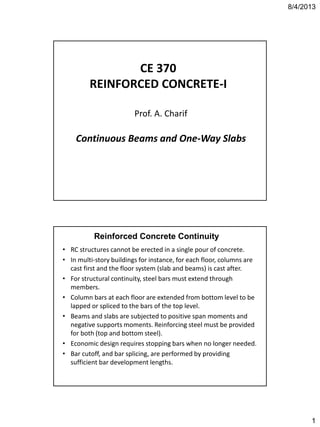
1. 8/4/2013
1
CE 370
REINFORCED CONCRETE-I
Prof. A. Charif
Continuous Beams and One-Way Slabs
Reinforced Concrete Continuity
• RC structures cannot be erected in a single pour of concrete.
• In multi-story buildings for instance, for each floor, columns are
cast first and the floor system (slab and beams) is cast after.
• For structural continuity, steel bars must extend through
members.
• Column bars at each floor are extended from bottom level to be
lapped or spliced to the bars of the top level.
• Beams and slabs are subjected to positive span moments and
negative supports moments. Reinforcing steel must be provided
for both (top and bottom steel).
• Economic design requires stopping bars when no longer needed.
• Bar cutoff, and bar splicing, are performed by providing
sufficient bar development lengths.

2. 8/4/2013
2
Beam / Slab Reinforcement
(Note column splicing)
Reinforced Concrete Continuity
Construction of Columns
for Next Floor
un MM 
Demand and Capacity Moment Diagrams
• Steel reinforcement is provided so that design capacity is
greater than or equal to the ultimate moment (demand):
• It is very convenient to represent demand and capacity
moments in a single diagram, illustrating bar cutoff.
• As required steel is on tension side, it is better for RC
structures to draw moment diagrams on the tension face
• For beam bending, positive span moment is on the bottom
face, and negative supports moments are on the top face.

3. 8/4/2013
3
• Capacity moment diagram greater than demand diagram.
• It shows required bar number and bar cutoff location.
• Demand diagram is an envelope curve from many load
combinations.
Demand and Capacity Moment Diagrams
Load cases and load combinations
• In RC structures, loading is applied as distributed or
concentrated forces and moments.
• Load cases to consider:
• Dead load - Live load - Wind load - Earthquake load
• Last two (wind and earthquake) present in some regions only.
• Codes define appropriate load combinations for design.
• This chapter focuses on Dead and Live load cases with the
following SBC ultimate load combination:
• Ultimate load = 1.4 x Dead load + 1.7 x Live load
• Usually dead and live loads are applied as area loads (kN/m2)
with values obtained from loading codes such as SBC-301.
• Wall line loads on beams (kN/m) may also be considered

4. 8/4/2013
4
Load transfer mechanism
• Dead and live loads applied in each floor are
transferred to the supporting beams, which transfer
them to the supporting columns before reaching the
structure foundations.
• Load transfer to beams may vary according to the
type of slab (one way or two way slab).
• Some beams may act as normal beams and be
supported by other beams which then act as girder
beams.
• Footing and column loads are cumulated from the
above floors.
Load patterns
• Dead load is permanent and applied on all parts of the
structure.
• Live load is variable and may be applied on selected
parts only.
• Design is performed for maximum values of internal
forces (moments, shear forces…).
• The structure must be analyzed for many combinations
with different live load applications to obtain maximum
effects.
• Influence lines may be used to determine the locations
of the parts to be loaded by live loads.

5. 8/4/2013
5
Influence lines for a six span continuous beam
Load patterns
• It is not easy to draw influence lines for complex structures,
but from the previous simple example, SBC, ACI and other
codes give simple guidelines for maximum effects:
1. For maximum negative moment and maximum shear force in
internal supports, apply live load on the two adjacent spans
to the support only.
2. For maximum positive span moment and maximum negative
moment in external supports, apply live load on alternate
spans.
• The various load combinations will produce envelope curves
for shear force and bending moment diagrams.

6. 8/4/2013
6
Envelope curves from many load combinations
General slab behavior
• Slab behavior is described by (thin or thick) plate
bending theory, which is a complex extension of beam
bending theory.
• Plates are structural members with one dimension
(thickness) much smaller than the other two.
• Beams are members with one dimension (length)
much greater than the other two.
• Beams and plates have specific bending theories
derived from general elasticity.
• Plate bending is more complex and involves double
curvature and double bending.

7. 8/4/2013
7
General slab behavior
45o
Ln1
45o
A B
C D
Ln2
Ws Ln2 / 2 Ws Ln2 / 2
Yield line model
Long beam load Short beam load
• Codes of practice allow use of simplified theories for slab
analysis, such as the yield line theory.
• In a rectangular slab panel, subjected to area load and
supported by edge beams, load is transferred from the slab to
the beams according to yield lines with 45 degrees.
• Long beams will receive trapezoidal load
• Short beams will be subjected to triangular load.
way-Two0.2
spanShort
spanLong
:If
way-One0.2
spanShort
spanLong
:If


One-Way Slabs and Two-Way Slabs
• In general loads are transferred in both directions (two-way
action)
• If the long beams are much longer than short beams, triangular
loads on short beams will become negligible.
• Loads are then considered to be transferred to long beams only.
This is called one-way action.
• Structural slabs are classified as one-way slabs or two-way slabs.
• Limit on length ratio between the two types is fixed by most
codes (SBC and ACI) as:

8. 8/4/2013
8
0.2
spanShort
spanLong

A
B
C
D
E
1 2 3
1-m slab strip
Types of one-way slabs
One way solid slab with beams and girders
• For each panel, aspect ratio
greater or equal to two:
• Slab supported by beams which
rest on columns or girders
• Analysis and design of 1-m strip
• Design results generalized to slab
• Shrinkage (temperature) steel
provided in other direction.
• Slab strip modeled as continuous
beam with beams as supports
Typical joist (rib)
Vertical section
bw S
bf
hw
hf
Void or hollow
block (Hourdis)
Joist (ribbed) slab
• Joists (Ribs) are closely spaced T-beams. Space between ribs
may be void or filled with light hollow blocks called “Hourdis”
• Joist slab very popular and offers many advantages (lighter, more
economical, better isolation).

9. 8/4/2013
9
A B
C D
One way slab with beams in one direction only
• In this case the loads are transferred to the supporting
beams whatever the aspect ratio.
Elastic analysis versus
approximate RC code methods
• Continuous beams and one way slabs can be analyzed using
standard elastic analysis methods (indeterminate structures).
• Codes such as SBC and ACI provide approximate and simplified
methods for analysis for these structural parts.
• These methods can be used if conditions are satisfied.
• Code methods offer advantages over elastic analysis:
 They are simpler to use
 They consider various loading patterns (presence of live load
on selected spans)
 They allow for partial fixity of external RC supports (in
elasticity, a support either pinned or totally fixed).

10. 8/4/2013
10
ACI / SBC coefficient method of analysis
• ACI / SBC method (coefficient method) is used for
analysis of continuous beams, ribs and one-way slabs.
• It allows for various load patterns with live load applied
on selected spans.
• Maximum shear force and bending moment values are
obtained by envelope curves.
• It allows for real rotation restraint at external supports,
where real moment is not equal to zero.
• Elastic analysis gives systematic zero moment values at all
external pin supports.
• Coefficient method is more realistic but valid for standard
cases on conditions.
• Use the method whenever conditions are satisfied.
• Elastic analysis used only if conditions of the code
method are not satisfied.
Conditions of application of ACI / SBC method
2.1
),(Min
),(Max
1
1



ii
ii
LL
LL
DLLL 3







2
)( 2 n
uvunumu
l
WCVlWCM
Ln = L – 0.5 (S1 + S2)
Ln
1. Two spans or more
2. Spans not too different. Ratio of two adjacent spans less than or equal to 1.2
For two successive spans (i) and (i+1), we must have :
3. Uniform loading
4. Unfactored live load less or equal to three times unfactored dead load, that is:
5. Beams with prismatic sections
Ultimate bending moment and shear force are given by:
ln is the clear length
Wu is the ultimate uniform load

11. 8/4/2013
11
ACI / SBC coefficient method of analysis







2
)( 2 n
uvunumu
l
WCVlWCM
• For shear force, span positive moment and external
negative moment, ln is the clear length of the span
• For internal negative moment, ln is the average of
clear lengths of adjacent spans.
• Cm and Cv are the moment and shear coefficients
given by next Table
• Moment coefficients given for each span at supports
(negative) and at mid-span (positive)
• Shear coefficients given at both ends (supports)
a/ Unrestrained end
More than 2 spans
Cm
-1/24 (16)*
Cv
-1/9 -1/9 -1/24 (16) *
+1/14 +1/14
1.0 1.15 1.01.15
Cm
-1/24(16)*
Cv
-1/10 -1/11 -1/11 -1/11 -1/11 -1/11
+1/14 +1/16 +1/16
1.0 1.0 1.0 1.0 1.0 1.01.15
b/ Integral end
More than 2 spans
c / Integral end
with 2 spans
* : The exterior negative moment depends on the type of support
If the support is a beam or a girder, the coefficient is: -1/24
If the support is a column, the coefficient is: -1/16
Cm
0
Cv
-1/10 -1/11 -1/11 -1/11 -1/11 -1/11
+1/11 +1/16 +1/16
1.0 1.0 1.0 1.0 1.0 1.01.15
ACI / SBC coefficient method of analysis

12. 8/4/2013
12
ACI / SBC coefficient method of analysis







2
)( 2 n
uvunumu
l
WCVlWCM

2
momentnegativeInternal
spanof
momentnegativeExternal
momentPositive
forceShear
Right
n
Left
n
n
nn
ll
l
ll








Coefficient Method: Integral end – More than two spans
External span Internal span
Locations External support Span
Internal
support
Internal
support Span
Internal
support
Moment
Coeff. Cm
-1/24 (Beam support )
1/14 -1/10 -1/11 1/16 -1/11-1/16 (Column support )
Shear Coef. Cv 1.0
* 1.15 1.0
* 1.0
ACI / SBC coefficient method of analysis
Coefficient Method: Integral end –Two spans
External span 1 External span 2
Locations External support Span
Internal
support
Internal
support Span
External
support
Moment
Coeff. Cm
-1/24 (Beam support )
1/14 -1/9 -1/9 1/14
-1/24
-1/16 (Column support ) -1/16
Shear Coef. Cv 1.0
* 1.15 1.15
* 1.0

13. 8/4/2013
13
Coefficient Method: Unrestrained end – More than two spans
External span Internal span
Locations
External
support Span
Internal
support
Internal
support Span
Internal
support
Moment
Coeff. Cm
0 1/14 -1/10 -1/11 1/16 -1/11
Shear
Coeff. Cv
1.0
*
1.15 1.0
*
1.0
* : The coefficient method does not give any value for mid-span
shear. However for shear design, it is safer to consider live load
applied on half span only, which gives a shear at mid-span equal to:
ACI / SBC coefficient method of analysis
LLu
nLu
uL ww
Lw
V 1.7loadliveFactored:,
8
2/ 
Reinforced concrete design
• Standard methods of RC design are also used for slabs,
with some particularities:
 Minimum steel for slabs is different from that in beams
 Design results are expressed in terms of bar spacing
 Maximum bar spacing must not be exceeded
 Concrete cover in slabs = 20 mm
 Stirrups are generally not required and shear checks
are performed to verify the slab thickness

14. 8/4/2013
14
CE 370
REINFORCED CONCRETE-I
Prof. A. Charif
Analysis and design of one-way
solid slabs with beams and girders
Analysis and design of one-way solid
slabs with beams and girders
A
B
C
D
E
1 2 3
1-m slab strip
0.2
spanShort
spanLong

For each panel aspect
ratio is greater than or
equal to two :

15. 8/4/2013
15
One way solid slab with beams and girders
• Slab is supported by beams which are supported by columns or
by girders
• Analysis and design of 1-m slab strip is then performed in main
direction and design results are generalized all over the slab.
• Shrinkage (temperature) steel provided in other direction
• Slab strip model is a continuous beam with supports as beams.
• Coefficient method of analysis used if conditions are satisfied.
• Standard flexural RC design methods used to determine
required reinforcement.
• Concrete cover = 20 mm, and stirrups are not used in slabs.
• Design results are expressed in terms of bar spacing.
• Minimum steel / maximum spacing requirements must be met.
Steps for analysis / design
of one-way solid slab (1-m strip)
• (1) Thickness: Determine and check minimum thickness using
ACI/SBC Table
• Minimum thickness must be determined for each span and final
value is the greatest of them
• If thickness unknown choose value greater or equal to minimum
• If thickness given, check that it is greater or equal to minimum
• If actual thickness greater or equal to minimum thickness, no
deflection check is required.
• A thickness less than minimum may be used but deflections must
then be computed and checked.

16. 8/4/2013
16
Simply
supported
One end
continuous
Both ends
continuous Cantilever
Solid one-
way slab
L / 20 L / 24 L / 28 L / 10
Beams
or ribs
L / 16 L / 18.5 L / 21 L / 8
 
LDu
LscD
www
mLLwmSDLhw
7.14.1
11

 
Table 9.5(a): Minimum thickness for beams (ribs) and
one-way slabs unless deflections are computed and checked
(2) Loading: Determine the dead and live uniform loading on
slab-strip (kN/m) using given area loads (kN/m2) for live load
and super imposed dead load as well as the slab self weight:
uc VV 
Steps for analysis / design
of one-way solid slab (1-m strip)
• (3) Analysis: Use coefficient method if conditions are satisfied.
Determine values of ultimate moments and shear forces for
each span at both supports and mid-span, using appropriate
clear lengths and coefficients.
• (4) Flexural RC design: Perform RC design starting with
maximum moment value. Determine required steel area and
check minimum steel and maximum spacing.
• (5) Shrinkage reinforcement: Determine shrinkage
(temperature) reinforcement and corresponding spacing
• (6) Shear check: Perform shear check:
If not checked, increase thickness and repeat from step (2)
• (7) Detailing: Draw execution plans

17. 8/4/2013
17
Example: One-way solid slab with beams / girders
4.0m
4.0m
4.0m
4.0m
8.2 m 8.1 m
A
B
C
D
E
1 2 3
1-m slab strip
MPaf
mkNMPaf
y
cc
420:Steel
/24,25:Concrete 3'

 
mkNwwall /4.14
Beams are in X-direction
Girders are in Y-direction
Panel ratio = 8.1/4 or 8.2/4 > 2
Beam/Girder section is
300 x 600 mm
Column section: 300 x 300 mm
Superimposed dead load :
SDL = 1.5 kN/m2
Live load : LL = 3.0 kN/m2
External beams / girders
support a wall load:
mkNw
w
wall
wallwall
/4.140.43.00.12
HeightThickness

 
All external beams and girders support a wall of 0.3 m
thickness and 4 m height with a unit weight of 12 kN/m3.
Wall loading is a line load (kN/m) and is part of dead
load. The wall line load is :
Wall loading on beams

18. 8/4/2013
18
Simply
supported
One end
continuous
Both ends
continuous Cantilever
Solid one-
way slab
L / 20 L / 24 L / 28 L / 10
Beams
or ribs
L / 16 L / 18.5 L / 21 L / 8
required)checkdeflectionno(170Take67.166
86.142
28
4000
28
:)continuousends(Both:3and2Spans
67.166
24
4000
24
:)continuousend(One:4and1Spans
min
min
min
mmhmmh
mm
L
h
mm
L
h



Solution of one-way solid slab example
Slab strip modeled as a continuous beam with four equal spans
Step 1: Thickness Use Table 9.5(a) for hmin
 
mkNwww
mkNmLLw
mkNw
mSDLhw
LDu
L
D
scD
/912.127.14.1:loaduniformUltimate
/0.310.31:striponloadLive
/58.5
1)5.1170.024(1:striponloadDead



 
• Step 2: Loading
• Area loading (SDL and LL) is assumed to be
applied on all floor area.
• Strip load (kN/m) = Slab load (kN/m2) x 1 m
(Use consistent units)

19. 8/4/2013
19







2
)( 2 n
uvunumu
l
wCVlwCM
mln 7.3
2
3.0
2
3.0
0.4:spansallFor 
• Step 3: Analysis
• All conditions of ACI/SBC coefficient method are satisfied.
(Discuss topic)
• ln is the clear length wu is the factored uniform load
• For shear force, span positive moment and external negative
moment, ln is the clear length of the span
• For internal negative moment, ln is the average of clear lengths of
the adjacent spans.
• Cm and Cv are moment and shear coefficients given by tables.
• Because of symmetry, we give results for the first two spans only.
First Span (external) Second Span (internal)
L (m) 4.0 4.0
Ln (m) 3.7 3.7
wu (kN/m) 12.912 12.912
Moment coeff. Cm -1/24 1/14 -1/10 -1/11 1/16 -1/11
Ln (m) 3.7 3.7 3.7 3.7
Moments (kN.m) -7.37 12.63 -17.68 -16.07 11.05 -16.07
Shear coeff. Cv 1.0 1.15 1.0 1.0
Ln (m) 3.7 3.7 3.7 3.7
Shear forces (kN) 23.89 27.47 23.89 23.89
2
7.37.3 
2
7.37.3 







2
)( 2 n
uvunumu
l
wCVlwCM
Analysis results for first two spans (symmetry)
Note that the external negative moment coefficient is (-1/24)
because the slab is supported by beams.

20. 8/4/2013
20
RC-SLAB1 software gives the following output:
 005.0controlioncheck tensand003.0,,
85.0
:Compute
)(Maxwith
7.1
4
11
85.0
2
coverstirrupsnoand20Cover
1
'
min2'
'











tt
c
ys
ss
u
n
c
n
y
cs
b
c
cda
c
bf
fA
a
A,ρbdA
bd
M
R
f
R
f
f
bd
A
d
hdmm




2
2
1.113
4
12
144
2
12
20170 mmAmmd b  
Section dimensions of strip: b =1000 mm, h = 170 mm
Assume a 12-mm bar diameter. Steel depth and one bar area are:
It is always better to start RC design with maximum moment value
(discuss)
• Step 4: Flexural RC design
• RC design of a rectangular section with tension steel only

21. 8/4/2013
21
RC design for interior negative moment Mu = 17.68 kN.m
OK005.005289.0
7289.7
7289.7144
003.0003.0
9728.7
85.0
5696.6
5696.6
85.0
35.332:useWe
0.30617010000018.0420
420if
420
0018.0
420if0018.0
350to300if0020.0
:slabsinsteelMinimum
35.3321441000002308.0
002308.0and94736.0:findWe
1
'
2
2
min
min
2























c
cd
mm
a
cmm
bf
fA
a
mmA
mmAMPaf
MPaf
f
bh
MPafbh
MPafbh
A
mmbdA
R
st
c
ys
s
sy
y
y
y
y
s
s
n




mm12@300:usesteel,For top
spacingmm300auseWe
300)300,1702(Min)300,2(Min
:isslabsfordirectionmaininspacingMaximum
3.340
35.332
1.1131000
:isspacingBar
max






mmmmhS
mm
A
bA
S
s
b
(Discuss spacing and bar diameter,
if S >> Smax then bar diameter may be reduced).
RC design for interior negative moment Mu = 17.68 kN.m

22. 8/4/2013
22
mm300@12
mm300@12
RC design for positive span moment Mu = 12.63 kN.m
• We find As = 235.85 mm2 which is less than the
minimum value of 306 mm2
• We thus use As = Asmin = 306 mm2
• with 300 mm spacing (Controlled by Smax)
• (we find S = 369.6 mm)
• So we use (bottom steel)
• Design for exterior negative moment Mu = 7.37 kN.m
• Since minimum steel controlled the previous moment
value of 12.63 kN.m, it certainly controls a smaller
moment value.
• So we use (top steel at external supports)
mm10@250:steelshrinkageforusethusWe
300)300,1704(Min)300,4(Min
:issteelshrinkageforspacingMaximum
5.256
0.306
5.781000
:isSpacing
max





mmmmhS
mm
A
bA
S
s
b
• Step 5: Shrinkage reinforcement
• Shrinkage steel (in secondary slab direction) is
equal to minimum steel.
• Ashr = Asmin = 306 mm2
• We use a smaller diameter of 10 mm
• Thus Ab = 78.5 mm2

23. 8/4/2013
23
• Step 6: Shear check
2stepfromrepeatandthicknessslabtheincreaseWe
beamsinasstirrupsprovidenotdotwe,If:Note
OKisShear0.90120x75.0
0.1201200001441000
6
25
6
:concreteofstrengthshearNominal
SFD)previoussee(47.27
2
7.3
912.1215.1
:(1.15)luelargest vatheuseweequal,arespansallSince
1.15or1.0eitherisCoeffcient
2
:isforceshearultimatethemethod,tcoefficientheUsing
75.0with:check thatmustWe
'
uc
uc
c
c
u
v
n
uvu
uc
VV
VkNV
kNNbd
f
V
kNV
C
l
wCV
VV





















Ln1 Ln2 Ln3
Ln1 /4
Max (0.3Ln2 ,0.3Ln3)Max (0.3Ln1 ,0.3Ln2)
Min. 150 mm
Bottom steel
12@300
Shrinkage steel
10@250
Top steel
12@300
• Step 7: Detailing
• The design results must be presented in appropriate
execution plans providing all information about various
reinforcements as well as the development lengths.
• Following ACI / SBC provisions may be used :

24. 8/4/2013
24
RC-SLAB1 Software
• The software performs all checks, analysis and
design. The final design output is:
4.0
4.0
4.0
4.0
8.2 m 8.1 m
A
B
C
D
E
1 2 3
lt
Transfer of loading from slab to beams
Uniform beam load is transferred
from the slab according to the
beam tributary width lt
The tributary width is computed
using mid-lines between beams.
For edge beams lt must include
all beam width and any slab
offset.
ml
ml
t
t
15.2
2
3.0
2
4
:EandAbeamsedgeFor
0.4
2
4
2
4
:DC,B,beamsinternalFor


loadbeamDirect
)(kN/mloadSlab(kN/m)loadBeam 2

 tl

25. 8/4/2013
25
4.0
4.0
4.0
4.0
8.2 m 8.1 m
A
B
C
D
E
1 2 3
lt
Transfer of loading from slab to beams
The five beams have two spans
each and are supported either by
girders (beams B, D) or by
columns (beams A, C, E)
Beams A and E are subjected to a
wall load of 14.4 kN/m
Beam dead load must include
beam web weight and any
possible wall load.
wallbwbwctscbD
tbL
whblhSDLw
lLLw


 )(
:isloaddeadBeam
:isloadliveBeam
mkNw
mkNw
w
mkNw
mkNw
mmmhhh
bL
bD
bD
bL
bD
sbbw
/45.615.23
/493.29
4.1443.03.02415.2)17.0245.1(
:loadwalltosubjectedE)and(AbeamsedgeFor
/0.1243
/416.2543.03.0244)17.0245.1(
:areloadsliveanddeadD),orC(B,beaminternalsFor
43.0430170600
:isthicknesswebBeam






hf = hs
bw = b
hw = h - hf
bf
wallbwbwctscbDtbL whblhSDLwlLLw   )(
Transfer of loading from slab to beams

26. 8/4/2013
26


















t
fw
n
w
f
t
fw
n
f
l
hb
l
b
b
l
hb
l
b
widthtributaryBeam
6
span)shortest(
12
Min:sectionL
widthtributaryBeam
16
span)shortest(
4
Min:sectionT
hf = hs
bw =b
hw = h - hf
bf bf
Effective beam section
• Because of beam-slab
interaction, the effective beam
section is:
• T-section for internal beams
• L-section for edge beams.
Steps for analysis / design of beams
4.0
4.0
4.0
4.0
8.2 m 8.1 m
A
B
C
D
E
1 2 3
lt
1. Thickness
2. Loading
3. Analysis
4. Flange width
5. Flexural design
6. Shear design
7. Detailing

27. 8/4/2013
27
mkNw
mkNwmkNw
bu
bLbD
/9824.55
/0.12/416.25


OKthereforeismm600ofthicknessactualThe
24.443
5.18
8200
:givesm)(8.2spanlargestThe
5.18
continuousendonehavespansBoth
min
min
mmh
L
h


• Step 2: Loading (Uniform loads were determined earlier)
Analysis and design of internal beam B
• The beam has two spans (8.2 m and 8.1 m) and is supported by
the three girders (1, 2 and 3).
• Step 1: Thickness , use table 9.5 (a)
mkNM
M
ll
wM
u
u
nn
buu
.31.383
)85.7(9824.55
9
1
29
1
momentnegativeInternal
:Example
2
2
21







 

• Step 3: Analysis
• All conditions of the coefficient method are satisfied.
• Clear lengths are 7.9 m and 7.8 m respectively.
• For internal negative moment average clear length 7.85 m is used
• Moment coefficients and envelope diagrams are shown.

28. 8/4/2013
28
First Span (external) Second Span (external)
L (m) 8.2 8.1
Ln (m) 7.9 7.8
wu (kN/m) 55.9824 55.9824
Moment coeff. Cm -1/24 1/14 -1/9 -1/9 1/14 -1/24
Ln (m) 7.9 7.9 7.8 7.8
Moments (kN.m) -145.58 249.56 -383.31 -383.31 243.28 -141.92
Shear coeff. Cv 1.0 1.15 1.15 1.0
Ln (m) 7.9 7.9 7.8 7.8
Shear forces (kN) 221.13 254.30 251.08 218.33
2
8.79.7 
2
8.79.7 







2
)( 2 n
uvunumu
l
wCVlwCM
Analysis results for beam B
Note that the external negative moment coefficient is (-1/24)
because the beam is supported by girders (beams).
RC-SLAB1 output
• Coefficient method
does not give any
shear coefficient at
mid-span
• For shear design,
mid-span shear force
is taken equal to :
LLu
Lu
nLu
uL
ww
w
Lw
V
1.7
loadliveFactored:
8
2/



29. 8/4/2013
29
• Step 4: Flange width
• The effective flange width is
mmb
mmm
mmxhb
mm
l
b
f
fw
n
f
1950
40004widthtributaryBeam
30201701630016
1950
4
7800
span)shortest(
4
Min












2
'
min 54254230000333.0
4.1
,
4
Max mmdb
ff
f
A w
yy
c
s 









• Step 5: Flexural RC design
• Accurate design: as a T-section
• Approximate safe design: as a rectangular section (ignoring
flange overhangs)
• Compute required steel and compare to minimum steel:
T-section design for positive moment
 
control-ioncheck tensand,strainsteel,axisneutral,
85.0
Compute
valueminimumthetocomparedbemust then)(areasteelTotal
1
with
7.1
4
11
85.0
:momentforsectionrrectangulaasdesignedWeb
2
,
85.0
,,
section-Fsection-Wsection-T:Decompose
)(in webblocknCompressioIf
)(sectionrrectangulaaasDesign
)(flangeinblocknCompressioIf
2
85.0:capacitynominalflangefullCalculate
webin theorflangein theblocknCompressio
st'
22'
'
'
'





c
bf
fA
a
AA
M
M
dbdb
M
R
f
R
f
dbf
A
MMM
h
dfAM
f
hbbf
AAAAMMM
haMM
, hb
haMM
h
dhbfM
wc
ysw
sfsw
nf
u
ww
wu
wu
c
wu
y
wc
sw
nfuwu
f
ysfnf
y
fwfc
sfsfswsnfnwn
funff
f
funff
f
ffcnff





































30. 8/4/2013
30
mmd
d
hd s
b
54210
2
16
40600
2
cover 
Assume bar diameter 16 mm and stirrup diameter 10 mm,
Cover = 40 mm , Steel depth is then :
• Design for interior negative moment Mu = 383.31 kN.m
• Rectangular and T-section designs give the same result:
• As = 2152.53 mm2 requiring 11 bars (one top layer in the flange)
• For the rectangular beam, one layer can contain five bars only and
for 11 bars, three layers are required.
• Re-design is required (after correcting the steel depth)
• It turns out that twelve bars are required (5 + 5 + 2).
Flexural RC design
• Design for positive span moment Mu = 249.56 kN.m
• Approximate rectangular section design: As = 1324.8 mm2 (7 bars)
• Accurate T-section design: As = 1232.3 mm2 (7 bars)
• Recall minimum steel is 542 mm2
• Beam web can only have 5 bars in one layer. Two layers are thus
required.
• RC design should be repeated by correcting effective steel depth.
• RC-SLAB1 software performs all successive design corrections by
checking bar spacing and updating number of layers.
• Two layers (5 bars in first and two bars in second) turn out OK.
Flexural RC design

31. 8/4/2013
31
RC-SLAB1 design output (as T-section or as Rectangular section)
Giving numbers of top and bottom bars, with bar cutoff
Step 6: Shear design
We perform shear design for the longest span (8.2 m) with higher
shear force value. Maximum shear at interior support with Cv = 1.15
kN
l
wCV n
buvu 3.254
2
9.7
9824.5515.1
2
:supportinteriorAt 1













LLu
nLu
uL
ww
Lw
V
1.7with
8
:spanMid 2/



32. 8/4/2013
32
63
Ln/2 = 3.95 md
VuL/2
Vud
Vu0
 
  kNV
VV
L
d
VV
kN
L
wV
kN
L
wV
m.mmd
ud
uLu
n
uud
n
LuuL
n
uu
17.222145.203.254
9.7
542.02
3.254
2
:sectionCritical
145.20
8
9.7
127.1
8
3.254
2
15.1
5420542:depthSteel
2/00
2/
0







Step 6: Shear design - Continued
Concrete nominal shear strength is :
64
kNNdb
f
V w
c
c 5.135135500542300
6
25
6
'

requiredareStirrups8125.50
2
:trequiremenStirrup
OKSection17.222125.5085.13575.055
:checkadequacySection


ud
c
uduc
VkN
V
kNVVkNV


Distance x0 beyond which stirrups are not required is :
mmm
VV
VVL
x
uLu
cun
3433433.3
145.203.254
5.13575.05.03.254
2
9.75.0
2 2/0
0
0 

















Step 6: Shear design - Continued

33. 8/4/2013
33
65
  (a)0.271600,5.0Min
875.304317.222
:spacinggeometryMaximum
1
max mmmmds
kNVV cud

 
mms
b
fA
f
s
mm
dn
An =
w
yv
c
s
v
7.659
300
42008.157
0.3,
25
0.16
Min
0.3,
0.16
Min:spacingsteelMinimum
08.157
4
100
2
4
2:legstwoStart with
2
max
'
2
max
2
2


















 

• This distance x0 is smaller than half-span. Stirrups are thus
required over a distance :
mmx
L
xL n
st 3433
2
,Min 00 






Step 6: Shear design - Continued
66
mm
V
V
dfA
s
c
ud
yv
5.222
10005.135
75.0
17.222
54242008.157
:spacingstirrupRequired 3
max 












 
spacingmm200auseWe
mm50ofmultiplesasvaluesspacingselectusuallyWe
)byd(controlle220
,,Mins:spacingAdopted
5.222:spacingstirrupRequired
7.659:spacingsteelMinimum
0.271:spacingmaximumGeometry
:summarytrequiremenspacingMaximum
3
max
3
max
2
max
1
max
3
max
2
max
1
max






smms
sss
mms
mms
mms
Step 6: Shear design - Continued

34. 8/4/2013
34
67
mmm
VV
VVL
x
kN
s
dfA
VV
mms
sss
uLu
uun
yv
cu
766766.0
145.203.254
9.2083.254
2
9.7
2
:isvalueforceshearthisoflocationThe
9.208
1000
1
542
250
42008.157
5.13575.0
:isforceshearingCorrespond
spacing)geometrymaximumtoding(correspon
250spacingsecondachooseWe
,,limits
threetheofanyexceednotdoesitprovidedincreasedbemaySpacing
2/0
20
2
2
2
2
3
max
2
max
1
max


































Step 6: Shear design - Continued
68
The total number of stirrups with first spacing is :
533.4
2
1
200
766
2
1
2
1
1
2
12
1
1121  n
s
x
nx
s
snxLs
mmLLR
mm
s
snLLLR
sst
ssst
25339003433
900
2
200
2005
2
12
1
11112


The number of stirrups with spacing s2 is :
1113.10
250
2533
2
2
2
2  n
s
R
n
The first stirrup is at a distance s1/2 = 100 mm. Four more
stirrups are needed to cover this distance x2 (= 766 mm)
The remaining distance for spacing s2 is :
Step 6: Shear design - Continued

35. 8/4/2013
35
69
Step 6: Shear design - Summary
Stirrups required over a distance Lst = 3433 mm (less than half-span)
Use of two-leg 10 mm stirrups as follows:
1. First stirrup at s1/2 = 100 mm, and then four stirrups with spacing
s1 = 200 mm (until 900 mm = Ls1)
2. Eleven stirrups with s2 = 250 mm (until Ls1 + Ls2 = 3650 mm)
Step 6: Shear design - Summary

36. 8/4/2013
36
Ln1 Ln2 Ln3
Ln1 /4
Max (Ln2/3 ,Ln3/3)Max (Ln1/3 ,Ln2/3)
Min. 150 mm
Bottom steel
Top steel
• Step 7: Detailing
• Similar to one way slab, except that there is no shrinkage steel,
stirrups are present, bar number is given instead of bar spacing.
ACI / SBC guidelines for beams and ribs
Ln1 Ln2 Ln3
Ln1 /4
Max (Ln2/3 ,Ln3/3)Max (Ln1/3 ,Ln2/3)
Min. 150 mm 7D16
4D16 12D16
• Step 7: Detailing

37. 8/4/2013
37
RC-SLAB1 design output can be used to draw execution plans
with a more economical reinforcement layout
• Internal beam D : Similar to beam B
• Internal beam C :
 Same tributary width of 4 m, but supports are columns
 Moment coefficients at external supports are -1/16 instead of
-1/24.
• External beam A or E :
 Smaller tributary width of 2.15 m.
 Supports are columns. Moment coefficients at external
supports are -1/16 instead of -1/24
 Dead load must include wall load of 14.4 kN/m.
 Effective section of the external beam is an L-section.
Analysis and design of other beams

38. 8/4/2013
38
Girder loading (uniform and concentrated)
Girders are subjected to
uniform load as well as
concentrated forces transferred
from supported beams.
The concentrated force
transferred by a beam to a
girder depends on the girder
tributary width, determined by
mid-lines between the girders.
4.0
4.0
4.0
4.0
8.2 m 8.1 m
A
B
C
D
E
1 2 3
lt
Girder loading (uniform and concentrated)
mll
bll
ttn
gttn
3.0

Girder tributary width is
determined by mid-lines
between the girders.
In order to avoid duplication
of the beam-girder joint
weight, the clear tributary
width ltn must be used.
It is obtained by subtracting
the girder width:
4.0
4.0
4.0
4.0
8.2 m 8.1 m
A
B
C
D
E
1 2 3
lt
ml
m
tn 85.7
15.8
2
1.8
2
2.8


ml
.
..
tn 95.3
254
2
30
2
28


ml
.
..
tn 90.3
204
2
30
2
18



39. 8/4/2013
39
4.0
4.0
4.0
4.0
8.2 m 8.1 m
A
B
C
D
E
1 2 3
Girder loading (uniform and concentrated)
Girders are supported by
columns. The three girders
(1, 2, 3) have two equal
spans each. Beams A, C, E
are also supported by
columns. So only beams B
and D transfer concentrated
forces to the girders.
m0.844  m0.844 
Girder model:
Girder concentrated force = Beam uniform loadx Clear tributary width
tnbLLtnbDD
gttntnbeam
lwPlwP
blllwP


:Live:Dead
with
ggL
wallggcggD
bLLw
whbbSDLw


:Live
:Dead 
Girder loading (uniform and concentrated)
The uniform load includes girder self weight, superimposed dead
load and live load applied on the girder width, as well as any possible
wall load :

40. 8/4/2013
40
mkNw
mkNw
kNP
kNP
gL
gD
L
D
/9.03.03:Live
/77.46.03.0243.05.1:Dead
:loading)wallsupporting(notgirderon theloadUniform
2.9485.70.12:Live
5156.19985.7416.25:Dead
:2girderto(D)BbeamfromedtransferrforceedConcentrat




Girder loading (uniform and concentrated)
Girder analysis
• Girders are analyzed and designed as beams (same steps)
• With the presence of concentrated forces applied on the girder,
one of the conditions of the coefficient method is not satisfied.
• Girder analysis must therefore be performed using standard
elastic analysis.
• Alternatively, concentrated forces may be transformed to
equivalent uniform loading in order to use the coefficient
method. This is possible in some simple cases only.
• This transformation may be performed on the basis of keeping
the same maximum bending moment or the same maximum
shear force.
• First transformation required for flexural analysis and design
• Second transformation required for shear analysis and design

41. 8/4/2013
41
2
,
8
:loaduniformEquivalent
2
,
4
:forceedConcentrat
:loadinguniformequivalentunder theand
forceedconcentratunder theforceshearandmomentMaximum
max
2
max
maxmax
wL
V
wL
M
P
V
PL
M
ww
PP


Transformation of concentrated forces to
equivalent uniform load
• Example: Simply supported beam subjected to concentrated
mid-span force P
L
P
w
wLP
L
P
w
wLPL
wL
V
wL
M
P
V
PL
M
ww
PP




22
:forcesshearmaximumEquating
2
84
:momentsmaximumEquating
2
,
8
:loaduniformEquivalent
2
,
4
:forceedConcentrat
2
max
2
max
maxmax
Transformation of concentrated forces to
equivalent uniform load

42. 8/4/2013
42
• Loads are transferred to columns from beams and girders
connected to them.
• These loads cause axial compression forces as well as bending
and shearing in both X-Z and Y-Z planes.
• Column internal forces may be determined by structural analysis.
• Column axial forces are cumulated through all floors.
• At each floor column axial force may be determined using
tributary width or tributary area concept.
• Column moments may be determined using moment distribution
method by isolating the column end with its connected members.
Transfer of loads to columns
• The axial force in each floor may be determined using
the preceding load transfer mechanism.
• The total column force may be computed from the
forces acting on the supported beams and girders using
the tributary width concept for each beam and girder.
• It may also be determined using the tributary area.
• Column tributary area At is determined using mid-lines
between column lines only (not beam lines).
Axial forces on columns

43. 8/4/2013
43
4.0
4.0
4.0
4.0
8.2 m 8.1 m
A
B
C
D
E
1 2 3
   

tiiwallitiwiwiictscD
tL
lwlhbAhSDLP
ALLP
,)(:Dead
:Live

• Column tributary areas are
shown by red lines
• Dead force includes area
loading as well the self
weight of the webs of all
beams and girders in the
tributary area.
• It also includes possible
walls.
Axial forces on columns
4.0
4.0
4.0
4.0
8.2 m 8.1 m
A
B
C
D
E
1 2 3
Axial forces on columns
2
2
2
2.65
2
0.8
2
0.8
2
1.8
2
2.8
:C2columnInternal
82.33
2
3.0
2
0.8
2
1.8
2
2.8
:E2columnEdge
64.17
2
3.0
2
0.8
2
3.0
2
2.8
:A1columnCorner
:areasbutarycolumn triSelected
mA
mA
mA
t
t
t








































44. 8/4/2013
44
Axial forces on columns
   

tiiwallitiwiwiictscD
tL
lwlhbAhSDLP
ALLP
,)(:Dead
:Live

• For beams / girders inside the tributary area, the total web self
weight and total wall load is considered : αi = 1
• For beams / girders with axis on the border of the tributary
area, only half is considered : αi = 0.5
• lti is the member length inside the tributary area.
• In order to avoid duplication of beam-girder joint weights,
clear lengths must be used for the beams and full lengths for
the girders.
Axial force in internal column C2
   

tiiwallitiwiwiictscD
tL
lwlhbAhSDLP
ALLP
,)(:Dead
:Live

• Tributary area = 65.2 m2
• Column C2 supports Beam C and Girder 2 and half of the
beams B and D.
• Clear distance of Beams (B, C, D) is : 8.15 - 0.3 = 7.85 m
• Distance of Girder 2 is : 8 m
• Substitution gives the following axial forces on Column C2 :
 
kNP
P
kNP
D
D
L
19.437
85.75.085.75.085.7843.03.0242.65)17.0245.1(:Dead
6.1952.650.3:Live




45. 8/4/2013
45
Axial force in internal column C2
 
kNP
P
kNP
D
D
L
19.437
85.75.085.75.085.7843.03.0242.65)17.0245.1(:Dead
6.1952.650.3:Live



• These forces may also be obtained from beams and girders
connected to the column using tributary widths.
• Column C2 is connected to Beam C and Girder 2.
• The concentrated force on the column is obtained from the
uniform load on beam C and girder 2 as well as the concentrated
forces on girder 2.
• These beam and girder forces have been determined before.
Axial force in internal column C2
50 % of the concentrated
forces transferred from beams
B and D to girder 2 are then
transferred to column C2.
before.asresultsameobtain theWe
19.4375156.1990.877.485.7416.25
any)(ifWallsforcesGirder
:isforceedconcentratDead
D
2
D
kNP
lwlwP tDtn
C
D



46. 8/4/2013
46
• Moments in columns may be determined in each direction using
moment distribution method on a simplified model where the
column joint (top or bottom) is isolated with all the members
connected to it. The other member ends are assumed to be fixed.
• Depending on the floor (intermediate or last), four possible
different cases can be met:
Computation of column moments using
moment distribution method
(a)
(b) (c) (d)
• Only beams (and girders) are loaded.
• The maximum moment in the column joint occurs when the
unbalanced moment is maximum, that is when one beam is loaded
by dead and live load and the other beam loaded by dead load only.
• It is recommended to load the longest beam with dead and live load.
• Cases (a) and (c) with one beam only lead to higher unbalanced
moments on the joint.
• Case (a) is the worst one as the unbalanced moment is resisted by
two members only.
Computation of column moments using
moment distribution method
(a)
(b) (c) (d)

47. 8/4/2013
47
Computation of column moments using
moment distribution method
• We consider the more general case (d) with four members.
• The beams are subjected to two different uniform loads and
two different concentrated forces at their mid-span.
• Considering clockwise direction as positive, the fixed end
moments at A resulting from loads in beams AB and AC are :
AB C
D
E
P2
P1
W2
W1
812812
)()(:AatmomentUnbalanced
812
)(,
812
)(
2
2
21
2
1
2
2
21
2
1
ACACABAB
A
ACABA
ACAC
AC
ABAB
AB
LPLwLPLw
M
FEMFEMM
LPLw
FEM
LPLw
FEM



Computation of column moments using
moment distribution method
AB C
D
E
P2
P1
W2
W1
812812
2
2
21
2
1 ACACABAB
A
LPLwLPLw
M 
• It is clear that this moment will be maximum when
one beam is fully loaded while the other is only
subject to dead load.
• Case (a) is in fact the worst as the unbalanced moment
is maximum with one beam fully loaded and the part
going to the column is maximum since two members
only are connected to the joint

48. 8/4/2013
48
Computation of column moments using
moment distribution method
• To put joint A in equilibrium, an opposite moment (-MA) must
be added and distributed between all members connected to
joint A according to their distribution factors.
• The distribution factor of member m in a joint, is equal to the
ratio of the member stiffness factor to the sum of all stiffness
factors of all elements connected to the joint. It represents the
part of the joint moment that the member supports.
• In any joint the sum of distribution factors of all elements
connected to the joint, is equal to unity.
 

























i i
m
i i
m
m
L
I
L
I
L
EI
L
EI
DF
4
4
Computation of column moments using
moment distribution method
 

























i i
m
i i
m
m
L
I
L
I
L
EI
L
EI
DF
4
4 I : Section moment of inertia
L : Span length.
E : Young’s modulus
The moments in the columns
at joint A (top of column AD
and bottom of column AE)
are therefore:
AEADACAB
AE
AAE
AEADACAB
AD
AAD
L
I
L
I
L
I
L
I
L
I
MM
L
I
L
I
L
I
L
I
L
I
MM































































49. 8/4/2013
49
AB C
D
E
W2
W1
Numerical application
Moment in intermediate floor columns
• We consider column C2 in an intermediate floor in
X-direction with loading coming from beam C
• We load the longest span (8.2 m) with ultimate
load while the shortest is loaded with factored
dead load only.
mkNw
mkNw
/58.35416.254.1
/98.550.127.1416.254.1
2
1


The fixed end moments at the column joint A and the resulting
unbalanced joint moment are :
mkNFEMFEMM
mkN
Lw
FEM
mkN
Lw
FEM
ACABA
AC
AC
AB
AB
.141.119534.194675.313)()(
.534.194
12
1.85.35
12
)(
.675.313
12
2.898.55
12
)(
22
2
22
1







AB C
D
E
W2
W1
Numerical application
Moment in intermediate floor columns
Assuming a column height of 3.5 m and
recalling beam section (0.3 x 0.6 m) and
column section (0.3 x 0.3), the member
stiffness factors are :
 
  34
3
34
3
34
4
10666667.6
1.8
12/6.03.0
10585366.6
2.8
12/6.03.0
1092857.1
5.3
12/3.0
m
L
I
m
L
I
m
L
I
L
I
AC
AB
AEAD
































50. 8/4/2013
50
Numerical application
The moments in the top
and bottom columns at
joint A are :
AEADACAB
AE
AAE
AEADACAB
AD
AAD
L
I
L
I
L
I
L
I
L
I
MM
L
I
L
I
L
I
L
I
L
I
MM






























































mkNMM AEAD .43.13
666667.6585366.692857.192857.1
92857.1
141.119 


If we load both beams with the same ultimate load, the unbalanced
moment would almost vanish and be caused only by the minor
difference in the span lengths. The resulting column moments
would be 0.85 kN.m only.
• Consider column C1 in the roof in X-direction :
• The out of balance moment and column moment
are thus :
A
B
D
W1
mkNM
mkNFEMM
AD
ABA
.055.71
585366.692857.1
92857.1
43.356
.675.313)(




• This moment in an edge (or corner) column in the roof, is more
than five times greater than the previous one in an internal
column and intermediate floor.
• Corner and edge columns in roof are subjected to higher moments
than other columns.
• Corner columns in roof are subjected to higher biaxial moments
Moments in roof columns

51. 8/4/2013
51
CE 370
REINFORCED CONCRETE-I
Prof. A. Charif
Analysis and design of joist slabs
Typical joist (rib)
Vertical section
bw S
bf
hw
hf
Void or hollow
block (Hourdis)
Analysis and design of joist slabs
• Joists (Ribs) are closely spaced T-beams which are supported by
transverse beams resting on girders or columns.
• Joist slab very popular and offers many advantages (lighter, more
economical, better isolation).
Space between ribs may be
void or filled with light hollow
blocks called “Hourdis”

52. 8/4/2013
52
bw S
bf
hw
hf
Void or Hourdis
Analysis and design of joist slabs
ACI / SBC conditions on joist dimensions
mmS
mm
S
h
bh
mmb
f
ww
w
800:Spacing
50
12/
:thicknessFlange
5.3:thicknessWeb
100:widthWeb







• ACI / SBC codes specify that concrete shear strength may be
increased by 10 % in joists.
• Usually stirrups are not required in joists, but are used to hold
longitudinal bars.
• It is therefore recommended to consider stirrups when computing
longitudinal steel depth.
Sbb wf  :widthFlange
• Analysis and design of joist slabs is thus equivalent to
analysis and design of a typical joist as a T-beam.
• Shrinkage reinforcement must then be provided in the
secondary direction
• Joist loading is determined with the flange width acting
as a tributary width. If Hourdis blocks are present, their
weight is added to dead load :
Analysis and design of joist slabs
jfjL
jwbjwjwcjfjfcjD
jf
bLLw
ShhbbhSDLw
b



:Live
)(:Dead
htBlock weigweightWebloadSlabloadDead


53. 8/4/2013
53
1. Thickness: Determine or check thickness
2. Geometry and Loading: Check joist dimensions and determine
loading, adding possible Hourdis weight to dead load
3. Analysis: Determine ultimate moments / shear forces at major
locations using coefficient method (if conditions are satisfied)
4. Flexural RC design: Perform RC design using standard methods
5. Shrinkage reinforcement: Determine shrinkage reinforcement
and corresponding spacing
6. Shear check: Perform shear check with Vc increased by 10%. If
not checked, stirrups must be provided.
7. Flange check: Part of the flange is un-reinforced. It must be
checked as a plain concrete member.
8. Detailing: Draw execution plans
Steps for analysis / design of joist slabs
Example of one-way joist slab
• Beams are in X-direction
• Girders are in Y-direction
• Joists in Y-directions
• Beams and girders have the
same section 300 x 600 mm
• Column section 300 x 300 mm
• Superimposed dead load is
SDL = 1.5 kN/m2
• Live load: LL = 3.0 kN/m2
• External beams / girders
support wall load of 14.4 kN/m
• Hourdis blocks used with unit
weight of 12 kN/m3
4.0
4.0
4.0
4.0
8.2 m 8.1 m
A
B
C
D
E
1 2 3
500
120120
50 250
Joist Data (mm)
MPaf
mkN
MPaf
y
c
c
420
/24
25
3
'





54. 8/4/2013
54
Simply
supported
One end
continuous
Both ends
continuous Cantilever
Solid one-
way slab
L / 20 L / 24 L / 28 L / 10
Beams / Ribs L / 16 L / 18.5 L / 21 L / 8
mmhhh
hhmmh
mm
L
h
mm
L
h
wf 30025050:knessjoist thicTotal
required)checkdeflectionno(OK,22.216
48.190
21
4000
21
:)continuousends(Both:3and2Spans
22.216
5.18
4000
5.18
:)continuousend(One:4and1Spans
minmin
min
min




Solution of joist slab example
Joist modeled as a continuous beam with four equal spans
Step 1: Thickness Use Table 9.5(a) for hmin
• Step 2: Geometry and Loading
• A) Geometry: Check joist dimensions
mmbSb
mmmmS
mm
mmS
mmh
mmbmmh
mmmmb
wf
f
ww
w
620120500:widthFlange
OK800500:Spacing
OK
50
67.4112/50012/
50:thicknessFlange
OK4201205.35.3250:thicknessWeb
OK100120:widthWeb








 



• B) Loading: Area loading (SDL and LL) applied on all floor area
kN/m614.87.14.1:Ultimate
kN/m86.162.03:Live
kN/m894.325.05.01225.012.02462.0)05.0245.1(
)(:Dead




jLjDju
jfjL
jD
jwbjwjwcjfjfcjD
www
bLLw
w
ShhbbhSDLw 

55. 8/4/2013
55







2
)( 2 n
uvunumu
l
wCVlwCM
mln 7.3
2
3.0
2
3.0
0.4:spansallFor 
• Step 3: Analysis
• All conditions of ACI/SBC coefficient method are satisfied.
(Discuss topic)
• ln is the clear length wu is the factored uniform load
• For shear force, span positive moment and external negative
moment, ln is the clear length of the span
• For internal negative moment, ln is the average of clear
lengths of the adjacent spans.
• Cm and Cv are the moment and shear coefficients given by
tables.
First Span (external) Second Span (internal)
L (m) 4.0 4.0
Ln (m) 3.7 3.7
wu (kN/m) 8.614 8.614
Moment coeff. Cm -1/24 1/14 -1/10 -1/11 1/16 -1/11
Ln (m) 3.7 3.7 3.7 3.7
Moments (kN.m) -4.91 8.42 -11.79 -10.72 7.37 -10.72
Shear coeff. Cv 1.0 1.15 1.0 1.0
Ln (m) 3.7 3.7 3.7 3.7 3.7 3.7
Shear forces (kN) 15.94 18.33 15.94 15.94
2
7.37.3 
2
7.37.3 







2
)( 2 n
uvunumu
l
wCVlwCM
Analysis results for first two spans (symmetry)
Note that the external negative moment coefficient is (-1/24)
because the joist is supported by beams.

56. 8/4/2013
56
RC-SLAB1
software
output
• Step 4: Flexural RC design
• Standard RC design of a T-section with concrete cover = 20 mm
• Assume bar diameter db = 12 mm and stirrup diameter ds = 8 mm
mmd
d
hd s
b
2668
2
12
20300
2
coverdepthSteel 
• RC design for internal negative moment Mu = 11.79 kN.m
• We find As = 121.88 mm2 requiring two 12 mm bars (we may
use two 10 mm bars).
• We perform RC design in other locations

57. 8/4/2013
57
RC-SLAB1 design output
• Step 5: Shrinkage reinforcement
• As in one way solid slabs, shrinkage steel (in secondary slab
direction) is equal to minimum steel.
• Ashr = Asmin = 0.0018 bh = 0.0018 x 1000 x 50 = 90 mm2
(we consider 1 m strip)
• We use a smaller diameter of 10 mm. Thus : Ab = 78.5 mm2
mm200@10:useWe
200)300,504()300,4(Min
:issteelshrinkageforspacingMaximum
2.872
90
5.781000
:isspacingingcorrespondThe
max





mmMinmmhS
mm
A
bA
S
s
b

58. 8/4/2013
58
• Step 6: Shear check
• We must check that concrete is sufficient to resist shear on its
own with its nominal shear strength increased by 10 % .
requiredstirrupsnoOK945.2175.0
33.18
2
7.3
614.815.1
2
:shearUltimate
26.2929260266120
6
25
1.1
6
1.1
:strengthshearconcreteNominal
'



ucc
n
juvu
w
c
c
VkNVV
kN
L
wCV
kNNdb
f
V

• Step 7: Flange check
• Flange part between webs must be checked as
a plain concrete member.
• We analyze a 1m strip.
• It is considered as fixed to both webs with a
length equal to spacing S = 500 mm = 0.5 m
• The section is b x hf = 1000 x 50 mm
• The ultimate uniform load is obtained from
slab loading:
S
w
  
   mkNmw
mLLhSDLmww fcsu
/88.8137.105.0245.14.1
17.14.11

 
mkN
Sw
Mu .185.0
12
5.088.8
12
22



• The maximum ultimate moment at fixed ends is:

59. 8/4/2013
59
• Step 7: Flange check – Continued
• As the member is un-reinforced, the nominal capacity must
consider concrete tension strength, as defined by SBC:
MPafct 5.37.0 '

OKisFlange.185.0
0.65:concreteplainFor
.948.0458.165.0
.458.1.1458333
6
501000
5.3
6
22






mkNMM
mkNM
mkNmmN
bh
M
un
n
f
tn




t
t
• The nominal moment for a rectangular section with
maximum stress equal to tension strength is:
• Step 8: Detailing
• Standard execution plans conforming to ACI / SBC provisions
for beams and ribs
Ln1 Ln2 Ln3
Ln1 /4
Max (Ln2/3 ,Ln3/3)Max (Ln1/3 ,Ln2/3)
Min. 150 mm
1D12
1D12 2D12

60. 8/4/2013
60
• Load is transferred by joists to
beams according to tributary
width lt as in one way solid
slabs
• Area load (kN/m2) used for
this purpose is equal to the
joist load (kN/m) divided by
the flange width.
• In order to avoid duplication of
the joist-beam joint weight, we
must use the beam clear
tributary width ltn, obtained by
subtracting the beam width.
4.0
4.0
4.0
4.0
8.2 m 8.1 m
A
B
C
D
E
1 2 3
bttn bll 
:beamofhutary widtClear trib
Transfer of loading from joist slab to beams
• Beams have two spans each
and are supported either by
girders or columns (beams A,
C, E)
• Beam dead load must include
possible wall load.
4.0
4.0
4.0
4.0
8.2 m 8.1 m
A
B
C
D
E
1 2 3
Transfer of loading from joist slab to beams
wallbbbctn
jf
jD
bD
tbL
wbSDLhbl
b
w
w
lLLw


:Dead
:Live
:loadingBeam

61. 8/4/2013
61
• Tributary widths and loads for
internal beams (B, C, D) are :
4.0
4.0
4.0
4.0
8.2 m 8.1 m
A
B
C
D
E
1 2 3
Transfer of loading from joist slab to beams
tbL
wallbbbctn
jf
jD
bD
lLLw
wbSDLhbl
b
w
w

 
mkNw
mkNw
mkNw
w
ml
ml
bu
bL
bD
bD
tn
t
/61.59:Ultimate
/1243:Live
/008.28:Dead
3.05.16.03.0247.3
62.0
894.3
7.33.00.4
0.4
2
4
2
4












• Because of the interaction between the beam and the slab, the
effective beam section is:
 T-section for internal beams
 L-section for edge beams.
• However with a small flange thickness (less than 80 mm), it is
recommended to use a rectangular section.
• Analysis and design of beams is performed using the same steps
as in one way solid slabs.
Effective beam section

62. 8/4/2013
62
• The following
figure is produced
by RC-SLAB1
software.
• It performs various
checks and gives
the analysis results
and diagrams.
Analysis and design of beam B
First Span (external) Second Span (external)
L (m) 8.2 8.1
Ln (m) 7.9 7.8
wu (kN/m) 59.61 59.61
Moment coeff. Cm -1/24 1/14 -1/9 -1/9 1/14 -1/24
Ln (m) 7.9 7.9 7.8 7.8
Moments (kN.m) -155.02 265.74 -408.15 -408.15 259.06 -151.12
Shear coeff. Cv 1.0 1.15 1.15 1.0
Ln (m) 7.9 7.9 7.8 7.8
Shear forces (kN) 235.47 270.79 267.36 232.49
2
8.79.7 
2
8.79.7 







2
)( 2 n
uvunumu
l
wCVlwCM
Analysis results for beam B

63. 8/4/2013
63
• This figure, also produced by RC-SLAB1 software, shows the
flexural design results with bar cutoff (considering a rectangular
section).
Analysis and design of beam B
Girder loading (uniform and concentrated)
• Girders are subjected to uniform loading and concentrated forces
transferred from supported beams just as in one-way solid slabs.
Concentrated forces on columns
• The axial forces in the columns may be determined, as in the case
of one-way solid slab, using the tributary area concept. The area
load is equal to the joist line load divided by the flange width.
• Dead force includes area loading as well self weight of the webs
of all beams and girders in the tributary area. It also includes
possible wall loads.
 
tL
tiiwallitiwiwiict
jf
jD
D
ALLP
lwlhbA
b
w
P

 
:Live
:Dead ,

64. 8/4/2013
64
RC-SLAB1 Software
Developed by Prof. Abdelhamid Charif
• This program performs analysis and design of RC one-way slabs
and continuous beams according to SBC and ACI codes.
• A powerful graphical interface is implemented .
• Both one-way solid slabs and joist slabs are considered.
• Inter-rib spaces may be void or contain “hourdis” blocks.
• The slab or the joist as well as supporting beams can be analyzed
and designed with automatic load transfer from slab to beams.
• Beam loading may include wall line load.
• Various code checks are performed (thickness, shear, flange, …).
• Both ACI / SBC coefficient method and elastic finite element
method can be used for the analysis.
• The coefficient method is used only if all conditions are satisfied.
• But even if these conditions are satisfied, the user can still choose
either method for comparison purposes
RC-SLAB1 Software
Developed by Prof. Abdelhamid Charif
• With the code coefficient method, envelope curves of the
moment and shear diagrams are generated and used in design.
• Beams may be designed using the original rectangular section or
the effective T-section / L-section (resulting from beam-slab
interaction) with automatic determination of flange width.
• The software delivers an optimum reinforcement pattern along
the model by performing appropriate bar cutoff.
• A powerful re-design algorithm allows checking and updating
bar / layer numbers and spacing.
• Both demand and capacity moment diagrams are produced.
• Shear design is performed for beams or ribs requiring it.
• Single stirrup spacing is produced for the critical section.
• For span design, variation of stirrup spacing is delivered.