Water Productivity Mapping (WPM) at various Resolutions (scales) using Remote Sensing - A proof of Concept Study in the Syr Darya River Basin in Central Asia - Xueliang Cai, Prasad S. Thenkabail, Alexander Platanov, Chandrashekhar M. Biradar, Yafit Cohen, Victor Alchanatis, Naftali Goldshlager, Eyal Ben-Dor, MuraliKrishna Gumma, Venkateswarlu Dheeravath, and Jagath Vithanage

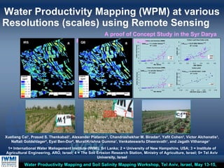
1. Water Productivity Mapping (WPM) at various Resolutions (scales) using Remote Sensing A proof of Concept Study in the Syr Darya River Basin in Central Asia Water Productivity Mapping and Soil Salinity Mapping Workshop, Tel Aviv, Israel, May 13-15, 2008 Xueliang Cai 1 , Prasad S. Thenkabail 1 , Alexander Platanov 1 , Chandrashekhar M. Biradar 2 , Yafit Cohen 3 , Victor Alchanatis 3 , Naftali Goldshlager 4 , Eyal Ben-Dor 5 , MuraliKrishna Gumma 1 , Venkateswarlu Dheeravath 1 , and Jagath Vithanage 1 1= International Water Management Institute (IWMI), Sri Lanka; 2 = University of New Hampshire, USA; 3 = Institute of Agricultural Engineering, ARO, Israel; 4 = The Soil Erosion Research Station, Ministry of Agriculture, Israel; 5= Tel Aviv University, Israel IRS QB kg/m 3 kg/m 3

2. Need, Scope, Context for WPM

4. Goals

6. Definition of WP

8. Study Area

9. A r a l S e a T o k t o g u l Kirgizstan Galaba Kuva Kazakhstan Tajikistan L a k e s B a s i n b o u n d a r i e s A d m i n i s t r a t i v e p r o v i n c e s R i v e r s C a n a l s # T e s t s i t e s Uzbekistan Irrigated area Water Productivity Mapping using Remote Sensing (WPM) The Syr Darya River Basin Source: IWMI, 2007

10. Galaba Kuva Kuva Scattered GT points in selected farm plots at Galaba study site Scattered GT points in selected farm plots at Kuva study site Water Productivity Mapping using Remote Sensing (WPM) Study Areas: Galaba and Kuva in the Syr Darya River Basin Photo Credit: Alexander Platanov Photo Credit: Alexander Platanov A r a l S e a T o k t o g u l Kirgizstan Galaba Kuva Kazakhstan Tajikistan L a k e s B a s i n b o u n d a r i e s A d m i n i s t r a t i v e p r o v i n c e s R i v e r s C a n a l s # T e s t s i t e s Uzbekistan Irrigated area

11. Dataset collection Dates: Satellite Sensor data and Groundtruth data

12. Water Productivity Mapping using Remote Sensing (WPM) Data Collection dates: Satellite sensor data and Groundtruth Data Source: IWMI, 2007

13. Characteristics of Satellite Sensor Data

14. Water Productivity Mapping using Remote Sensing (WPM) Characteristics of the Satellite Sensor Data Source: IWMI, 2007

15. MODIS (@ 250-500 m) Water Productivity Mapping using Remote Sensing (WPM) Satellite sensor Data Coverage Source: MODIS IRS P6 (@ 23.5m) ETM+ (@ 14-30m) Syrdariya Fergana Quickbird (@ 0.6-2 m) IKONOS (@ 1-4m) Hyperion (@ 30m) ALI (@ 30m)

16. Groundtruth Data Collection and Synthesis

17. Water Productivity Mapping using Remote Sensing (WPM) Illustration of Groundtruth Data Collection Photo Credit: Alexander Platanov Source: IWMI, 2007 0.69 kg/m 3 Water Productivity 4394.283333 m 3 /ha Water application 3.04 (ton/ha) Yield 1 Seed type * * Electrical conductivity (EM-38) * * Electrical conductivity (EM-38) * * Electrical conductivity (EC Meter) * (0 o C) Soil Temperature (EC meter) 4 (%) Soil Salinity * (text) Soil Type * (%) Soil Moisture 2 (grading) Crop Vigour 2 (grading) Crop Health (1-5) 1 Crop Growth Stage 3 Intensity Cropping 0.0015 (kg/m 2 ) Biomass Dry 0.01125 (kg/m 2 ) Biomass Wet 15 (plants/m 2 ) Crop Density 51 (mm) Crop Height 3 (%) Weed cover 0 (%) Water cover 90 (%) Soil cover 7 (%) Canopy Cover 0.12 (ratio) LAI Meter LAI 1399 (µmol m -2 s -1 ) LAI Meter PAR 0.017 (unitless) Average NDVI from NDVI Camera 280 (m) Elevation 07-May-2006 (num) English Date 68.84597 (num) Longitude 40.39519 (num) Latitude 2 No.Points 1 No.Visit 2 No.Field Cotton Crop Name Galaba Location G-C-F5-V01-02 (code) Unigue_Id 65 (num) SLNO value Unit Item

18. Water Productivity Mapping using Remote Sensing (WPM) Illustration of Groundtruth Data Collection Source: IWMI, 2007 Photo Credit: Alexander Platanov 0.692 kg/m 3 Water Productivity 4394 m 3 /ha Water application 3.04 (ton/ha) Yield 1 Seed type 103.2 * Electrical conductivity (EM-38) 154.4 * Electrical conductivity (EM-38) 0.88 * Electrical conductivity (EC Meter) 27.3 (0 o C) Soil Temperature (EC meter) 4 (%) Soil Salinity * (text) Soil Type 1.5 (%) Soil Moisture 3 (grading) Crop Vigour 4 (grading) Crop Health (1-5) 4 Crop Growth Stage 3 Intensity Cropping 0.496 (kg/m 2 ) Biomass Dry 1.104 (kg/m 2 ) Biomass Wet 12 (plants/m 2 ) Crop Density 400 (mm) Crop Height 2 (%) Weed cover 5 (%) Water cover 53 (%) Soil cover 40 (%) Canopy Cover 1.907 (ratio) LAI Meter LAI 830 (µmol m -2 s -1 ) LAI Meter PAR 0.579 (unitless) Average NDVI from NDVI Camera 282 (m) Elevation 02-Aug-2006 (num) English Date 68.84694 (num) Longitude 40.39447 (num) Latitude 3 No.Points 7 No.Visit 2 No.Field Cotton Crop Name Galaba Location G-C-F5-V07-03 (code) Unigue_Id 84 (num) SLNO Value Unit Item

19. Water Productivity Mapping using Remote Sensing (WPM) Groundtruth Data: Variables, Sample size, and Mean Values of the Variables Source: IWMI, 2007 b = the "watchdog" automated weather station was set up in Galaba site and the weather data was used for all crops. Note: a = Average value of vertical and horizontal EC. 355.2 4 158.9 4 80.57 2 293 5 Weirs mm Irrigation application E. Water applied measurements 151.8 5798 mm Rainfall 1.38 5798 KM/h Wind Speed 169.8 5798 (February-October) degree Wind direction 50 5798 station b % Relative humidity 22.1 5798 Automated weather Selsius degree Air temperature D. Meteorological variables for plant water use estimations or ET calculations 3.61 41 3.028 108 3.087 172 3.004 573 Eye estimation grading Crop vigor 3.78 41 3.231 108 3.291 172 3.164 572 Eye estimation grading Crop health 13.738 42 0.01 108 0.556 173 3.51 585 Eye estimation % Water cover 10.595 42 14.426 108 12.922 173 5.025 585 Eye estimation % Weed cover 343.077 39 18.213 97 253.837 172 21.133 577 Cut and counting plant/m 2 Crop density 18 6 11.95 15 16.9 9 12.55 36 Laboratory (weight) % Soil moisture 79.933 26 110.279 62 91.077 48 106.567 315 EM-38 a dS/m EC C. Variables to study the factors affecting Water Productivity 4.523 6 2.983 18 3.495 45 2.109 45 Laboratory ton/ha Yield 69.78 42 36.451 113 58.035 173 34.087 585 Eye estimation % Canopy cover 8.2 42 49.301 113 30.144 175 61.753 585 Eye estimation % Soil cover 610.244 41 920.88 108 569.535 172 453 576 Ruler mm Crop height 0.884 37 0.994 106 0.563 172 0.772 575 Cut and counting kg/m 2 Dry biomass 2.166 37 2.186 108 1.499 172 1.801 577 Cut and counting kg/m 2 Wet biomass 2.84 38 1.204 105 2.057 173 1.338 580 LAI meter - Leaf area index 957.868 38 960.429 105 1029 174 1060 580 LAI meter µmol m -2 s -1 PAR 0.602 43 0.571 105 0.622 166 0.487 566 NDVI camera - NDVI B. Crop variables for spectro-biophysicalield modeling - 2 - 6 - 15 - 15 Eye observation - Soil type - 43 - 116 - 191 - 585 Hand-held GPS degree Coordinate Rice Rice Maize Maize Wheat Wheat Cotton Cotton A. General Mean value Sample size Mean value Sample size Mean value Sample size Mean value Sample size Collecting method Unit Variable

20. WPM: methods

22. 1. Crop Type Mapping

23. 1a. Crop Type Mapping using IRS LISS 23.5 m time-series Data Source: IWMI, 2007 Legend Wheat Settlements Fallow land Galaba

24. LULC and the areas in Galaba site 1b. Crop Type Mapping using Quickbird 2.44 m single date for Galaba Source: IWMI, 2007 Photo Credit: Alexander Platanov Photo Credit: Alexander Platanov Photo Credit: Alexander Platanov Alfalfa Cotton Fallow Home garden Orchard Rice Settlements Legend 100.0 9924.5 Sum 17.8 1769.9 other 5.8 573.9 Settlement 3.6 361.8 Rice 0.0 1.4 Orchard 0.9 90.3 Home garden 18.7 1853.8 Fallow 44.5 4414.9 Cotton 8.7 858.5 Alfalfa % ha share Areas LULC

25. 2a. Spectro-Biophysical Models

26. Images: (1) IRS, (2) Quickbird Band reflectance as variable: (1) bands, (2) TBVI Dependent variable: (1) Wet biomass, (2) Dry biomass, (3) Yield, (4) LAI 2a. Spectro-Biophysicalield Models Different Types of Models bioDry = a * IRSbx ** b [ Log(BioDry) = Log(a) + b* Log(IRSbx) ] Power: bioDry = a * e ** (b* IRSbx) [ Log(BioDry) = Log(a) + b*IRSbx ] Exponential: bioDry = a + b * log(IRSbx) Logarithmic: bioDry = a + b * IRSbx + c * IRSbx^2 Quadratic: bioDry = a + b * IRSbx1 + c * IRSbx2 Multi-linear: bioDry = a + b * IRSbx Linear: Models and respective equations: (Dry biomass and IRS bands as example)

27. 2b. Best Models from all Model Types

28. A, Yield model using 2007 data B, Yield model using 2006 data C, ∑ NDVI camera is the accumulated NDVI derived using the hand hold NDVI camera for field data during 2006 D, Sample points of data from Quickbird for maize was inadequate E, Sample points of data from IRS for rice was inadequate Note: 2b. Spectro-Biophysicalield Models using IRS LISS 23.5m and Quickbird 2.44m Data Best Model R 2 values and Waveband combinations Source: IWMI, 2007 0.858 1,3; 3,4 Multi-linear 0.927 1, 3, 4 Multi-linear 8 QB 0.639 3, 4 Exp 0.499 3 Power 21 IRS LAI 0.867 1,2; 2,3; 3,4 Multi-linear 0.732 2, 4 Multi-linear 8 QB 0.812 1, 2 Exp 0.817 2 Power 21 IRS Dry Biomass 0.887 1,2; 2,3; 3,4 Multi-linear 0.772 2, 4 Multi-linear 8 QB 0.853 1, 2 Quadratic 0.838 2 Power 21 IRS Wet Biomass Alfalfa 0.234 2, 3 Quadratic 0.879 2, 4 Multi-linear 10 QB LAI 0.414 1,3; 2,3 Multi-linear 0.395 1, 2 Multi-linear 10 QB Dry Biomass 0.600 1,2; 2,4 Multi-linear 0.535 1, 2 Multi-linear 10 QB Wet Biomass Rice E 0.839 1,2; 2,3 Multi-linear 0.777 1, 3 Multi-linear 19 IRS LAI 0.903 2, 3 Power 0.928 2 Exp 17 IRS Dry Biomass 0.871 2, 3 Power 0.815 2 Power 19 IRS Wet Biomass Maize D 0.67 2, 3 Linear 12 IRS Yield 0.465 1,3; 2,3 Multi-linear 0.8 4 Quadratic 18 IRS LAI 0.309 3, 4 Quadratic 0.205 1 Quadratic 14 IRS Dry Biomass 0.678 1, 3 Quadratic 0.425 2 Quadratic 9 IRS Wet Biomass Wheat 0.610 3, 4 Linear 7 QB B 0.753 2, 3 Linear 14 IRS A Yield 0.574 2, 4 Quadratic 0.511 2, 4 Multi-linear 41 QB 0.725 1, 3 Power 0.634 3, 4 Multi-linear 135 IRS LAI 0.661 1, 2 Exp 0.521 2 Exp 41 QB 0.821 2, 3 Power 0.620 2 Power 136 IRS Dry Biomass 0.506 1,4; 3,4 Multi-linear 0.813 1, 4 Multi-linear 41 QB 0.834 2, 3 Power 0.697 2 Exp 140 IRS Wet Biomass Cotton R-square band combination Best model R-square band Best model sample size Sensor Parameter Crop Best indices Best bands crops using IRS LISS and Quickbird data (5-10% points sieved) Spectro-biophysical and yield models. The best models for determining biomass, LAI and yield of 5

29. 2c. Illustrative Plots of Best Models

30. Note: * the cotton yield model uses September 4, 2007 IRS LISS image. 2c1. Best Spectro-Biophysicalield Models Illustrative Examples for Cotton Crop Variables versus IRS LISS 23.5 m Data Source: Xueliang Cai, 2009

31. Note: * The best model for cotton wet biomass using Quickbird image ** The wheat yield model uses April 18, 2007 IRS LISS image. is WBMcotton = 17.416 - 0.685 * QBb1 - 0.163 QBb4 2c2. Best Spectro-Biophysicalield Models Illustrative Examples for Cotton, wheat, Maize versus Qucikbird and IRS indices Source: Xueliang Cai, 2009

32. 2c. Model Validation

33. Note : Twenty-five percent points were reserved for validation 2d. Spectro-Biophysicalield Model Validation Models evaluated for Cotton Crop using IRS LISS 23.5 m Data Source: Xueliang Cai, 2009

34. 2d. Frequency of Occurrence of Bands

35. Note: blue band only occur in Quickbird and swir only in IRS data An overwhelming proportion of the best models involved the use of indices rather than wavebands. The red and the near-infrared (NIR) bands, which are also required for computation of NDVI, were most frequently occurring. The green band follows closely. Blue band is not very critical in modeling crop variables. SWIR band 1 (see IRS in Table 1) was found, surprisingly, less important. 2e. Frequency of Occurance of Bands in Best Models Source: IWMI, 2007

36. 3. Extrapolation to Larger Areas

37. Wet biomass map (18-Jul-2006) Yield map Dry biomass map (18-Jul-2006) LAI map (18-Jul-2006) 3. Extrapolation to Larger Areas using IRS LISS 23.5 m using best models of cotton crop variables Source: IWMI, 2007 19.8 0 Legend (kg/m 2 ) 10.7 0 Legend (kg/m 2 ) 4.1 0 Legend (kg/m 2 ) 3.2 0 Legend (ton/ha)

38. 4a. Water use (ET actual ) using simplified surface energy balance Model (SSEBM)

39. ET act – the actual Evapotranspiration, mm. ET frac – the evaporative fraction, 0-1, unitless. ET 0 – reference ET, mm. T x – the Land Surface Temperature (LST) of pixel x from thermal data. T H /T C – the LST of hottest/coldest pixels. 4a. Water use (ET actual ) Water use is determined by multiplying Evaporative fraction by reference ET

40. 4b. ET frac.

41. 2006-04-24 2006-05-10 2006-06-11 2006-07-29 2006-08-14 2006-10-01 4b. ET fraction Evaporative fraction using Landsat ETM+ thermal data during crop growing season Source: IWMI, 2007 Legend unitless

42. 4c. ET ref.

43. 4c. ET reference Using Penman-Montieth Equation based on meteorological data Source: IWMI, 2007

44. 4d. ET act.

45. ET map for cotton field, average ET=512mm (Apr 15 – Oct 15, 2006) ET map for rice field, average ET=619mm (May 21 – Sept 28, 2006) 4d. ET actual ET actual = ET fraction * ET reference Water use of Irrigated Cotton versus Irrigated Rice crops Source: IWMI, 2007 905 150 Legend mm 769 165 Legend mm

46. 5. Water Productivity Maps (WPM)

47. (1) 5a. Water Productivity WP calculated in this study

48. WPM using IRS LISS 23.5 m and Quickbird 4 m 5b1. Water productivity maps (WPMs) at 2 Resolutions (Scales) Unit: kg/m 3 IRS QB Kg/m 3 Kg/m 3 Source: IWMI, 2007 0.4 17.9 0.1 2.4 >0.6 2.0 93.0 1.2 50.3 0.5-0.6 11.7 542.7 10.0 414.7 0.4-0.5 29.6 1370.0 33.4 1381.7 0.3-0.4 33.5 1550.7 34.4 1421.0 0.2-0.3 21.0 970.2 16.8 695.5 0.1-0.2 1.8 85.1 4.1 167.9 0-0.1 share (%) area (ha) share (%) area (ha) group Quickbird IRS 7776175 1.06 1.06 0 0.289 QB 74850 0.7 0.70 0 0.285 IRS No. Pixels Range Max Min Mean

49. (a) (b) Within field variability of water productivity derived from (a) Indian Remote Sensing (IRS) P6 and (b) Quickbird images Unit: kg/m 3 5b2. Water productivity maps (WPMs) at 2 Resolutions (Scales) IRS LISS 23.5 m versus Quickbird 2.44 m Source: IWMI, 2007 80.2 81 Area (ha) 134642 0.61 0.68 0.07 0.339 QB 1296 0.52 0.60 0.08 0.334 IRS No. Pixels Range Max Min Mean 0.68 0.07 Legend kg/m 3 0.68 0.07 Legend kg/m 3

50. Within field variability of water productivity derived from (a) Indian Remote Sensing (IRS) P6 and (b) Quickbird images (a) (b) Unit: kg/m 3 5b3. Water productivity maps (WPMs) at 2 Resolutions (Scales) IRS LISS 23.5 m versus Quickbird 2.44 m Source: IWMI, 2007 0.58 0.09 Legend kg/m 3 0.58 0.09 Legend kg/m 3 6.6 6.7 Area (ha) 11083 0.49 0.58 0.09 0.339 QB 107 0.38 0.50 0.12 0.334 IRS No. Pixels Range Max Min Mean

51. 5c. Water Productivity Scope for improvement With an average value of 0.3 kg/m 3 , the water productivity map shows explicit scope for improvement: where and how much. Source: IWMI, 2007 Legend <0.3 0.3-0.4 >0.4 Kg/m 3

52. 6. Factors Affecting Water Productivity

53. 6a. Factors Affecting WP Degree of influence of Various factors on WP variations within and between field as measured during field work Photo Credit: Alexander Platanov Photo Credit: Alexander Platanov Photo Credit: Alexander Platanov Photo Credit: Alexander Platanov Photo Credit: Alexander Platanov Land leveling Weeds 6% Salinity Water deficit 43% 31% 14% 7% Water logging

54. Quickbird NDVI (26-July-2006) IRS NDVI (18-July-2006) High salinity Low salinity 6c. Factors Affecting WP Degree of influence of Various factors on WP variations within and between field as measured during field work Photo Credit: Alexander Platanov Photo Credit: Alexander Platanov Source: IWMI, 2007 0.69 0.06 Legend unitless 0.69 0.06 Legend unitless

55. 6d. Factors Affecting WP Distinguish different levels of factors affecting WP using crop variables and spectral vegetation indices – soil salinity as example EC values were grouped into four groups indicating different levels of soil salinity. Mean TBVI values of the respective groups were plotted. Test of differences: Source: IWMI, 2007 AD,BD AB,AC,AD, BC,BD TBVI41 TBVI32

56. Note: # = Statistical tests of significance were conducted to determine significant differences between two groups of data. For example, A-B # indicates that IRS band 2 mean spectral reflectivity is significant different between moisture level A and B at 95% confidence level or higher 6d. Factors Affecting WP Distinguish different levels of factors affecting WP using crop variables and spectral vegetation indices Source: IWMI, 2007 AB,AC,AD,BC,BD AB,AC,AD,BD AB,AC,AD,BC,BD AD,BD AB,AC,AD,BC,BD AB,AC,AD,BD AB,AC,AD,BC,BD AB,AC,AD AB,AC, AD,BD AB,AC,AD,BD AB,AC, AD, BD, AB,AC, AD,BD, CD AB,AC, AD,BD AB,AC, AD,BD, CD AB,AC, AD, BD, CD TSS 0.284 0.316 0.132 0.109 0.192 0.215 0.024 11.805 22.638 15.428 14.641 0.345 0.777 0.926 0.355 70 x>=14 D 0.352 0.337 0.105 0.092 0.238 0.253 0.014 11.795 23.882 14.725 14.184 0.677 1.404 1.301 0.503 104 10<x<=14 C 0.431 0.363 0.076 0.080 0.291 0.291 0.004 11.616 25.005 13.771 13.650 0.919 1.966 1.523 0.557 90 6<x<=10 B [dS/m] 0.584 0.429 0.035 0.070 0.394 0.370 0.035 10.751 27.221 11.769 12.389 1.421 2.961 2.181 0.669 44 x<=6 A ECEM38 AD,BD AD,BD AD,BD AD,BD AD,BD AD,BC, BD AD,BC,BD AD,BC,BD AD,BC,BD AC AC,AD, BC,BD AD,BD TSS 0.285 0.304 0.118 0.089 0.193 0.222 0.029 12.639 23.743 16.099 15.111 0.425 0.945 0.919 0.408 45 x>=10 D 0.354 0.336 0.104 0.097 0.239 0.248 0.007 11.679 23.481 14.550 14.172 0.395 0.903 1.007 0.397 50 5<x<=10 C [%] 0.493 0.393 0.063 0.090 0.333 0.313 0.027 10.511 24.180 12.161 12.583 0.695 1.689 1.269 0.459 159 2<x<=5 B cover 0.473 0.380 0.062 0.082 0.319 0.306 0.020 11.080 24.830 12.811 13.075 0.728 1.785 1.290 0.477 191 x<=2 A Weed AB,AC AB,AC AB TSS 0.491 0.450 0.138 0.195 0.333 0.279 0.059 7.547 19.882 9.955 11.213 0.799 1.935 1.586 0.597 9 x>=5 C [%] 0.413 0.391 0.120 0.139 0.280 0.265 0.020 9.219 21.218 11.894 12.158 0.605 1.598 1.756 0.562 18 x<=5 B cover 0.469 0.378 0.064 0.081 0.317 0.306 0.017 11.136 24.846 12.955 13.133 0.787 1.829 1.335 0.491 537 x=0 A Water AB,AC AB AB,AC AB,AC AB,AC AB,AC AB BC AB,AC AB,BC BC AB,AC, BD,CD AB,AC, BD,CD AB,AC, BD,CD BD,CD TSS 0.416 0.351 0.074 0.070 0.281 0.287 0.004 12.052 25.299 14.165 13.901 0.308 0.822 0.720 0.347 34 x>40 D 0.467 0.376 0.063 0.077 0.315 0.308 0.014 11.448 25.476 13.333 13.408 0.940 2.052 1.393 0.495 200 20<x<=40 C [plant/m2] 0.503 0.393 0.056 0.085 0.340 0.318 0.029 10.675 24.625 12.166 12.656 0.835 2.059 1.488 0.524 261 10<x<=20 B density 0.355 0.345 0.112 0.104 0.240 0.250 0.009 11.001 22.611 13.926 13.554 0.360 0.790 1.062 0.443 77 x<=10 A Crop AB,BC AB,BC AB,BC,BD AC,AD,BC,BD AB,BC AB,BC AB,AD,BC,CD AC,AD,BD,CD AB,AC, AD,BC, BD AB,AD, CD AB # ,AD, CD Test of statistical significance (TSS) # 0.517 0.415 0.072 0.123 0.350 0.307 0.051 8.659 21.181 10.086 11.046 0.943 2.342 1.650 0.581 33 x>1.7 D 0.420 0.376 0.100 0.106 0.284 0.280 0.007 10.422 22.966 12.776 12.813 0.649 1.600 1.547 0.564 42 1.2<x<=1.7 C [descriptive] 0.620 0.433 0.009 0.063 0.419 0.380 0.053 10.778 27.406 11.261 12.230 0.802 1.816 1.272 0.480 75 x<=1.2 B moisture 0.452 0.371 0.069 0.081 0.305 0.299 0.012 11.348 24.891 13.323 13.387 0.781 1.811 1.337 0.487 417 x=1 A Soil SAVI TBVI43 TBVI42 TBVI41 TBVI32 TBVI31 TBVI21 IRSb4 IRSb3 IRSb2 IRSb1 Dry biomass (kg/m 2 ) Wet biomass (kg/m 2 ) LAI ( - ) NDVI ( - ) No. of samples Criterion Grade

57. Note: # = Statistical tests of significance on crop vigor and health were conducted to determine significant differences between two groups of data. For example, A-B # indicates that IRS band 2 mean spectral reflectivity is significant different between moisture level A and B at 95% confidence level or higher 6e. Factors Affecting WP Distinguish different levels of factors affecting WP using crop variables and spectral vegetation indices Source: IWMI, 2007 AC,AD,AE,BC,BD,BE,CD,CE AC,AD, AE,BC, BD,BE, CD,CE AC,AD, AE,BC, BD,BE, CD,CE AC,AD, AE,BC, BD,BE, CD AC,AD,AE,BC,BD,BE,CD,CE AC,AD,AE,BC,BD,BE,CD,CE AC,AD, AE,BC, BD,BE, CD,CE AD,AE, BD,BE, CD AC,AD,AE,BC,BD,BE,CD,CE,DE AC,AD,AE,BC,BD,BE,CD,CE AC,AD,AE,BD,BE,CD,CE AC,AD, AE,BC, BD,BE, CD,CE, DE AC,AD, AE,BC, BD,BE, CD, CE AC,AD,AE,BC,BD,BE,CD,CE,DE AC,AD,AE,BC,BD,BE,CD,CE,DE Test of statistical significance 0.703 0.479 0.003 0.060 0.474 0.430 0.063 10.162 29.452 10.318 11.509 1.715 3.593 2.772 0.783 31 best E 0.588 0.423 0.025 0.069 0.398 0.364 0.044 10.480 25.908 11.233 12.043 1.163 2.893 1.834 0.645 202 D 0.430 0.363 0.078 0.087 0.290 0.285 0.009 11.393 24.448 13.500 13.524 0.607 1.332 1.068 0.410 199 C 0.315 0.325 0.119 0.104 0.213 0.228 0.015 11.569 22.667 14.797 14.217 0.279 0.600 0.775 0.323 110 B [descriptive] 0.233 0.297 0.147 0.116 0.158 0.189 0.032 12.030 22.120 16.105 15.085 0.153 0.307 0.619 0.304 30 wrost A Crop health AC,AD,AE,BC,BD,BE,CD,CE,DE AC,AD, AE,BC, BD,BE, CD,CE, DE AC,AD, AE,BC, BD,BE, CD,CE, DE AC,AD, AE,BC, BD,BE, CD,CE AC,AD,AE,BC,BD,BE,CD,CE,DE AC,AD,AE,BC,BD,BE,CD,CE,DE AC,AD, AE,BC, BD,BE, CD,CE, DE AC,AD, AE,BC, BD,BE, CE AC,AD,AE,BC,BD,BE,CD,CE,DE AC,AD, AE,BC, BD,BE, CD,CE,DE AC,AD,AE,BC,BD,BE,CD,CE,DE AC,AD, AE,BC, BD,BE, CD,CE, DE AC,AD, AE,BC, BD,BE, CD,CE, DE AC,AD,AE,BC,BD,BE,CD,CE,DE AC,AD, AE,BC, BD,BE, CD,CE, DE Test of statistical significance # 0.810 -0.516 0.044 -0.047 0.547 0.480 -0.091 9.536 30.227 8.718 10.458 1.786 3.844 2.708 0.814 35 best E 0.608 -0.433 -0.021 -0.068 0.411 0.376 -0.047 10.453 26.524 11.139 12.000 1.258 3.099 1.987 0.666 131 D 0.478 -0.382 -0.063 -0.083 0.323 0.308 -0.020 10.978 24.587 12.645 12.945 0.720 1.642 1.189 0.466 246 C 0.319 -0.325 -0.116 -0.101 0.216 0.231 0.016 11.736 23.066 14.941 14.362 0.255 0.624 0.860 0.329 117 B [descriptive] 0.233 -0.290 -0.139 -0.107 0.157 0.189 0.033 12.291 22.235 16.226 15.164 0.201 0.399 0.568 0.280 40 wrost A Crop vigor SAVI TBVI43 TBVI42 TBVI41 TBVI32 TBVI31 TBVI21 IRSb4 IRSb3 IRSb2 IRSb1 Dry biomass (kg/m 2 ) Wet biomass (kg/m 2 ) LAI (-) NDVI (-) No. of samples Criterion Grade

59. Conclusions

61. Thanks www.iwmi.org