SlideShare una empresa de Scribd logo
1 de 70
PROJECT REPORT
On
COMPARISON STUDY BASED ON POWER ANGLE CALCULATION FOR ELECTRICAL
NETWORK STABILITY.SIMULATION.CASE STUDTY RWANDA NETWORK.
By
BALIRWANDA Jean Marie Vianney
Reg.No: UG 10102475
And IYAMUREMYE IRENE
Reg.No:10103654
Under the guidance of HAKUZWUMUREMYI Victor (MS)
Submitted to the DEPARTMENT OF <ELCTRICAL AND ELECTRONICS>
in the FACULTY OF APPLIED SCIENCES
in partial fulfillment of the requirement
for the award of the degree of
BACHELOR OF SCIENCE
In
Electrical and Electronics Engineering
NATIONAL UNIVERSITY OF RWANDA
FACULTY OF APPLIED SCIENCES
DEPARTMENT OF <ELECTRICAL AND ELECTRONICS>
October, 2011
ii
BONAFIDE CERTIFICATE
Certified that this project report titled comparison based on power angle calculation for
electrical network stability .Simulation case study Rwanda network is the bonafide work
of Mr./ Ms BALIRWANDA Jean Marie Vianney and IYAMUREMYE Iréné who carried
out the research under my supervision. Certified further, that to the best of my knowledge
the work reported herein does not form part of any other project report or dissertation on the
basis of which a degree or award was conferred on an earlier occasion on this or any other
candidate.
Eng. Victor HAKUZWUMUREMYI, Msc Eng. Ezechiel MANIRAGABA, Msc
Signature of Internal Guide/ Signature of External Guide/
Name: Name:
Submitted for University examination held in October 2011 at National University of Rwanda,
University Avenue, Butare, Rwanda.
iii
DECLARATION
We declare that, the project entitled, “comparison study based on power angle
calculation for electrical network stability ” is original work and has never been
submitted to any University or other Institutions of Higher Learning. It is our own
research whereby other scholar’s writings were cited and references provided. We thus
declare this work is ours and was completed successfully under the supervisor
HAKUZWUMUREMYI VICTOR.
BALIRWANDA Jean Marie Vianney
and
IYAMUREMYE Iréné
iv
ABSTRACT
This project deal with the ways in which we can transmit the maximum real power demand when
we have the interconnect system of different generators basing on power angle calculation for
electrical network stability. There are mains parameters that can cause the instability in network
such as the generator out of synchronism, current fluctuation in transmission line, many change
in loads, manual or automatically changes of excitation, irregularities in prime mover input,
inductive loads, and the faults in transmission line. Those parameters some of them affect power
angle such as inductive loads, reactive power, real power demand, and changes in load. To avoid
their effects to the power angle, in this project controlling real power, reactive power, and
voltage, current and inductive loads with Matlab simulator is its goal .To achieve the goal of this
project, the study in the change of power transfer for variations in transfer reactance and sending
end and receiving end voltages will be done, then the plot of graph for power angle characteristic
is made in order to see for which angle we have maximum power transfer in transmission line.
v
DEDICATION
This memoire is dedicated
To the Almighty God;
To my parents;
To my wife;
To my loved sister and brothers;
To all my friends.
BALIRWANDA J M V
vi
DEDICATION
To the Almighty God
To my late parents
To my brothers and sisters, regretted brother and sister
To my relatives, my best friends
All benefactors during my studies
IYAMUREMYE Iréné
vii
ACKNOWLEDGEMENT
First and foremost, t hanks to my forever loving and protective JESUS CHRIST, for the
gift of life and for His love to me.
I would like to thank my supervisor MSR HAKUZUMUREMYI VICTOR for his guidance ,
support, and patience throughout my research. MSR HAKUZUMUREMYI VICTOR is a
great teacher who has been an invaluable resource when I’ve needed to discuss a new
idea or clarify an old concept. It has truly been a pleasure to conduct research under his
guidance. Without his guidance,
I would have been lost. Special thanks go to all teachers who taught me from my primary
school up to now .
I also wish to thank the power engineering students that I have worked with in both
my own research group and others. I have thoroughly enjoyed discussing ideas with them
and gaining a variety of different perspectives.
Most importantly, I thank my parents, for their countless sacrifices in raising me and
supporting me in all my endeavors. They have always believed in me and encouraged
me to shoot for the stars. My thanks also go out to my sisters and brothers , whose
continuous love and support help me to persevere through the most arduous situations.
Lastly, I thank all my friends at Nyarubaka secondary school who give me the support in
different ways.
Thank you all.
BALIRWANDA J M V
viii
ACKNOWLEDGEMENT
My first thanks are due to almighty GOD who protected me during my research and my whole
period of my life especial during my studies. I would like also to acknowledge all those who
supported me to accomplish this project through its many stages. I really recognize the work of
Eng. Victor HAKUZWUMUREMYI (MSc), my supervisor who, despite his multiple attributions
and many responsibilities, sat down and give me the right direction of this project. All those
hours he has spent on the issue of this work are recognized, his efforts is appreciated.
I would like to extend my gratitude to the teaching staff of faculty of applied sciences especially
those of the department of electrical and electronics engineering, option of electrical power
engineering and the National University of Rwanda in general, for facilitating my studies at the
university.
I have got many friends and colleagues like JMV BALIRWANDA, Gaspard MUNYANGANIZI
and Juvénal NSENGIYUMVA who have made special contributions to this work in many ways
whether scientifically or psychologically. I must thank all my classmates who helped me getting
at this level throughout six years of studies at the university.
Special thanks go to my sister and my brother who really have been incomparable people during
my studies since many years ago, their support has been for great important in my studies. I end
up by recognizing the love, help and support of my relatives.
IYAMUREMYE Iréné
ix
TABLE OF CONTENTS
BONAFIDE CERTIFICATE..........................................................................................................ii
DECLARATION...........................................................................................................................iii
ABSTRACT................................................................................................................................... iv
DEDICATION................................................................................................................................ v
DEDICATION............................................................................................................................... vi
ACKNOWLEDGEMENT............................................................................................................vii
ACKNOWLEDGEMENT...........................................................................................................viii
TABLE OF CONTENTS............................................................................................................... ix
LIST OF TABLES........................................................................................................................ xii
LIST OF FIGURES .....................................................................................................................xiii
LIST OF ABREVIATIONS ......................................................................................................... xv
CHAPTER I: GENERAL INTRODUCTION................................................................................ 1
1.1 Background........................................................................................................................... 1
1.2 Problem statement................................................................................................................. 2
1.3 Objective of the study........................................................................................................... 2
1.4 Benefits of the study ........................................................................................................... 3
1.5 Project aim ............................................................................................................................ 3
1.6 The research method............................................................................................................. 3
1.7 subdivision of the work......................................................................................................... 4
CHAPTER II: LITERATURE REVIEW ....................................................................................... 5
2.0 Introduction to power system stability.................................................................................. 5
x
2.1 Why the need for Power System Stability............................................................................ 5
2.2.1 Need for Classification................................................................................................... 6
2.2.2 Classification of Power System Stability....................................................................... 6
2.2.3 Voltage Stability .......................................................................................................... 10
2.2.4 Frequency Stability...................................................................................................... 11
2.3.2 Reactive power............................................................................................................. 12
2.3.3 Apparent power.......................................................................................................... 12
2.3.4 Power factor and power angle...................................................................................... 14
CHAPTER III: DETERMINATION OF POWER ANGLE CHARACTERISTIC OF
TRANSMISSION LINE............................................................................................................... 26
3.1 Introduction on a transmission line..................................................................................... 26
3.1.1Transmission line design information........................................................................... 26
3.1.2Transmission line models ............................................................................................. 27
3.1.3 The transmission line performance.............................................................................. 29
3.2 Determination of power angle characteristic of transmission line...................................... 30
3.2.1 Theory related to calculations of a transmission line................................................... 30
3.2.2 The simulation of the data for a transmission line....................................................... 31
3.2.3 Observation of the results for a transmission line........................................................ 32
3.2.4 Report of the results..................................................................................................... 34
CHAPTER IV: ITERPRETATIONS OF THE RESULTS .......................................................... 39
4.1 Introduction......................................................................................................................... 39
4.2 The discussion made on the results..................................................................................... 39
CHAPTER V: CONCLUSION AND RECOMMENDATIONS ................................................. 44
5.1. CONCLUSION.................................................................................................................. 44
5.2 RECOMMENDATIONS.................................................................................................... 45
xi
REFERENCES ............................................................................................................................. 46
APPENDIX 1...................................................................................................................................I
APPENDIX 2..................................................................................................................................II
APPENDIX 3................................................................................................................................ III
APPENDIX 4................................................................................................................................ IV
APPENDIX 5................................................................................................................................. V
xii
LIST OF TABLES
Table 3-1 Variation of and X with Vs=Vr=100 V.................................................................... 33
Table 3-2 variation of Vs and Vr with =30 deg. and X=520mH.............................................. 33
xiii
LIST OF FIGURES
Figure 2-1 Possible classification of power system stability into various categories and
subcategories................................................................................................................................... 6
Figure 2-2:First swing analysis for stable case............................................................................... 9
Figure 2-3:First swing analysis for unstable case........................................................................... 9
Figure 2-4 (a) the resistive load only............................................................................................ 13
Figure2-4 (b) reactive load only ................................................................................................... 13
Figure2-4 (c) resistive and reactive load....................................................................................... 14
Figure 2-5 Power triangles for (a) capacitive load and (b) inductive load ................................... 15
Figure 2-6 schematic of on machine against infinite bus diagram. .............................................. 15
Figure2-7 power angle curve ........................................................................................................ 17
Figure 2-8 Power angle characteristics at constant field excitation, illustrating determination of
steady state stability limit.............................................................................................................. 18
Figure2-9 Equivalent two-machine system .................................................................................. 20
Figure 2-10 Illustration of the graphical method for determination of stability limit. ................. 20
Figure 2-11 receiving end circle diagram, Vs=1.0 ....................................................................... 21
Figure 2-12 Power-angle Characteristic curve ............................................................................. 22
Figure2-13 Schematic of a system supplying a constant current load and phasor diagram. ........ 22
Figure 3-1 A distributed parameter model of a transmission line ................................................ 27
Figure 3-2 short transmission line................................................................................................. 28
Figure 3-3(a) Medium transmission line in П representation....................................................... 28
Figure 3-3 (b) Medium transmission line in T representation. ..................................................... 28
Figure 3-4 Long transmission line................................................................................................ 29
Figure 3-5 Short transmission line supplied with two sources ..................................................... 32
Figure 3-6 The power angle curve when the reactance x=70mH at the sending end of
transmission line. .......................................................................................................................... 34
Figure 3-7 The power angle curve when the reactance x=70mH at the receiving end of the
transmission line. .......................................................................................................................... 35
Figure 3-8 The power angle curve when the reactance x=520mH at the sending end of the
transmission line. .......................................................................................................................... 36
xiv
Figure 3-9 The power angle curve when the reactance x=520mH at the receiving end of
transmission line. .......................................................................................................................... 37
Figure4-2The simulated Data of a short transmission line. .......................................................... 41
Figure 4-3 Shows the displayer of the scope for the transmitted power for scope displayer 1; the
currents on the scope displayer 2 and voltage on the scope displayer 3 in function of time are the
same as the receiving end data...................................................................................................... 43
xv
LIST OF ABREVIATIONS
A: Ampere
AC: Alternative Current
HVDC: High Voltage Direct Current
Ir: current at the receiving end
Is: current at the sending end
MATLAB: Matrix Laboratory
MVA: Mega Volt Ampere
MVar: Mega Volt Ampere Reactive
P: True Power
Pe: electrical power
PF: Power factor
Q: Reactive Power
S: Apparent power
SCADA: Supervisory Control and Data Acquisition
V: Volt
Vr: Voltage at the receiving end
Vs: Voltage at sending end of the line
Wr: Maximum power received at the end of the line
xvi
Ws: Maximum power transmitted at the end of the line
β; ;∆’ : angles
1
CHAPTER I: GENERAL INTRODUCTION
1.1 Background
The development of the country need always the use of electricity that causes the growth of the
loads which are always the main cause of the low power factor (bad power angle), then this
cause the instability in a network. To get the solution of the lack of electricity the government
stakes out the new power plants in different area of the country. The purpose of this project is
one of the solutions of the instability in a network.
The stability of an electrical network is the ability of synchronous machine of a power system to
remain in synchronism after a very time of disturbance .Small disturbances are always present in
a power system ;for example there are many changes in load ,manual or automatic changes of
excitation ,irregularities in prime-mover input. Obviously these small disturbances cannot cause
loss of synchronism unless the system is operating at, or near its steady state stability limit.
Continuously electricity supply is conducted if only certain synchronous generators are ready to
supply. Once the generator is out of synchronism, significant voltage and current fluctuation is
occurred. These could initiate trouble in transmission line system .Consequently, a monitoring
system to ensure power steady state stability is required.
Power transmission steady state stability shows the maximum transmitted power.
Power transmission capacity of a generator group depends on power angle difference with
another generator group. The voltage instability phenomena and current fluctuation, which can
occur in both transmission systems and distribution systems, must be avoided in a network.
With the development of national economy and the improvement of people’s life in the county,
the load demands in distribution networks are sharply increasing. Like transmission networks,
the operation conditions of distribution networks are more and more close to the voltage stability
boundaries and current fluctuation in the network. The decline of voltage stability level is one of
important factors which restrict the increase of load served by distribution companies.
2
For example; in 1997, a voltage instability problem in a distribution network, which was
widespread to a corresponding transmission system, caused a major blackout in the Brazilian
system. Therefore, it is necessary to consider voltage stability constraints for planning and
operation of distribution systems in order to avoid the instability in network. Also, in 2009
Rwanda network has faced the same problem of instability of voltage which causes the
disturbance in network and the damage of different equipments. In this project, Emphasis will be
given to the network stability based on power angle calculation in which the system is described
by different equations using the different methods of calculations.
1.2 Problem statement
The main problem is that “what is the amount of the maximum power can be transmitted in an
interconnected system of generators? What is the role of the power angle in transmitting this
maximum power?’’
1.3 Objective of the study
1.3.1 General objective
 The general objective of this project is to study and to analyze different methods used in
power angle calculation for power system stability.
 To draw the power angle characteristic.
 To study the change in power transfer for variations in transfer reactance, and sending
end and receiving end voltages.
1.3.2 Specific objective
 To have a good value of power angle for a power system stability.
 Relationship between power angle and transmitting maximum power.
3
1.4 Benefits of the study
1.4.1 Personal benefits
This study will help me to master the skills learnt in power system stability analysis, power
control and correction of power factor for a network, will also help me to understand well the
simulation which will be used.
1.4.2 Community benefits
This project will show a good way of calculating power angle, the relationship between power
angle and transmitting maximum real power in a network.
1.5 Project aim
This project will show a good way of calculating power angle, and the relationship between
power angle and transmitting maximum real power in a network using different methods of
calculation for power angle and simulation.
1.6 The research method
The following approaches which include the methods used to obtain results were used in the
project. The relevant mathematics was studied in detail.
 A study was made of the theory of power system stability, power factor
calculations(power angle),real power ,reactive power and apparent power.
 Although a highly technical textbook related to power system stability, power angle
calculation or power factor, is available and is very good for the understanding of power
angle calculation phenomena and other sources, were found to be more useful in the
actual project method implemented during the power angle calculations and computer
simulations.
4
 The computer program used is Matlab simulator.
 Data were collected to computer the results of the case study.
1.7 subdivision of the work
This project will present the following points:
Chapter one will focus on the presentation of the general introduction to this project.
Chapter two will focus on the presentation of the theory of power system stability, real power,
reactive power, power angle.
Chapter three will focus on presentation of calculations related to power angle characteristic of
transmission line, using Matlab simulation.
Chapter four will present the interpretation of the results comparing with the theoretical values
for power angle characteristics of transmission line.
Chapter five will focus on recommendation and conclusion.
5
CHAPTER II: LITERATURE REVIEW
2.0 Introduction to power system stability
Power system stability denotes the ability of an electric power system, for a given initial
operating condition, to regain a state of operating equilibrium after being subjected to a
physical disturbance, with most system variables bounded so that system integrity is preserved.
Integrity of the system is preserved when practically the entire power system remains intact with
no tripping of generators or loads, except for those disconnected by isolation of the faulted
elements or intentionally tripped to preserve the continuity of operation of the rest of the system.
Stability is a condition of equilibrium between opposing forces; instability results when a
disturbance leads to a sustained imbalance between the opposing forces.
The power system is a highly nonlinear system that operates in a constantly changing
environment; loads, generator outputs and key operating parameters change continually. When
subjected to a transient disturbance, the stability of the system depends on the nature of the
disturbance as well as the initial operating condition.
2.1 Why the need for Power System Stability
The power system industry is a field where there are constant changes. Power industries are
restructured to cater to more users at lower prices and better power efficiency. Power systems are
becoming more complex as they become inter-connected.
Load demand also increases linearly with the increase in users. Since stability phenomena limits
the transfer capability of the system, there is a need to ensure stability and reliability of the
power system due to economic reasons.
6
2.2 Classification of Power System Stability
2.2.1 Need for Classification
The general principles of the classification are defined by Kundur in reference [1] According to
the reference; the classification of power system stability is based on the following
considerations:
-the physical nature of the resulting instability (related to the main system variable in which
instability can observed).
-the size of the disturbance considered (with influences the method of calculation and prediction
of stability).
2.2.2 Classification of Power System Stability
Figure 2-1 Possible classification of power system stability into various categories and
subcategories.
7
The following are descriptions of the corresponding forms of stability phenomena.
2.2.2.1 Rotor Angle Stability
Rotor angle stability is concerned with the ability of interconnected synchronous machines of a
power system to remain in synchronism under normal operating conditions and after being
subjected to a disturbance. It depends on the ability to maintain or restore equilibrium between
electromagnetic torque and mechanical torque of each synchronous machine in the system.
Instability that may result occurs in the form of increasing angular swings of some generators
leading to their loss of synchronism with other generators.
2.2.2.1.1 Small signal (or steady state) stability
Small signal (or steady state) stability refers to the stability of a power system subject to small
and gradual changes in load, and the system remains stable with conventional excitation and
governor controls. In today’s practical power systems, small signal stability is largely a problem
of insufficient damping of oscillations. The time frame of interest in small-signal stability studies
is on the order of 10 to 20 s following a disturbance
2.2.2.1.2 Large disturbance rotor angle stability or transient stability
Refers to the stability of a power system subject to a sudden and severe disturbance beyond the
capability of the linear and continuous supplementary stability control, and the system may lose
its stability at the first swing unless a more effective countermeasure is taken, usually of the
discrete type, such as dynamic resistance braking or fast valving for the electric energy surplus
area, or load shedding for the electric energy deficient area.
For transient stability analysis and control design, the power system must be described by
nonlinear differential equations.
8
2.2.2.1.2.1 Fundamentals of Transient Stability
Transient stability concerns with the matter of maintaining synchronism among all generators
when the power system is suddenly subjected to severe disturbances such as faults or short
circuits caused by lightning strikes, the sudden removal from the transmission system of a
generator and/or a line, and any severe shock to the system due to a switching operation.
Because of the severity and suddenness of the disturbance, the analysis of transient stability is
focused on the first few seconds, or even the first few cycles, following the fault occurrence or
switching operation. First swing analysis is another name that is applied to transient stability
studies, since during the brief period following a severe disturbance the generator undergoes its
first transient overshoot, or swing. If the generator(s) can get through it without losing
synchronism, it is said to be transient stable. On the other hand, if the generator(s) loses its
synchronism and cannot get through the first swing, it is said to be (transient) unstable.
There is a critical angle within which the fault must be cleared if the system is to remain stable.
The equal-area criterion is needed and can be used to understand the power system stability.
Before getting into detail discussion of the subject, some simple figures can be utilized to
graphically represent the difference between a stable case and an unstable case. In a stable case,
as shown in Figure 2-2, if the fault is cleared at 1t c second, or at angle 1cδ , where the area Aa
(area associated with acceleration of the generator) equals the area Ad (area associated with
deceleration of the generator). One can see that the angle reaches its maximum mδ at 1t c and
never gets greater than this value. In the unstable case, as shown in Figure 2-3, the fault is
cleared at 2t c second with the area Aa greater than the area Ad. Also, it is very clear that for an
unstable case, with the fault cleared at 2t c the angle keeps increasing and goes out-of-step, or
unstable, as shown in Figure 2-3.
9
Figure 2-2:First swing analysis for stable case
Figure 2-3:First swing analysis for unstable case
Transient stability depends on both the initial operating state of the system and the severity of
the disturbance. Usually, the disturbance alters the system such that the post-disturbance steady
state operation will be different from that prior to the disturbance.
10
2.2.3 Voltage Stability
Voltage stability is concerned with the ability of a power system to maintain steady voltages at
all buses in the system under normal operating conditions, and after being subjected to a
disturbance. Instability that may result occurs in the form of a progressive fall or rise of voltage
of some buses.
A run-down situation causing voltage instability occurs when load dynamics attempts to restore
power consumption beyond the capability of the transmission system and the connected
generation (Kundur, 1994; Taylor, 1994; Van Cutsem and Vournas,1998).While the most
common form of voltage instability is the progressive drop in bus voltages, the possibility of
overvoltage instability also exists and has been experienced at least on one system (Van Cutsem
and Mailhot, 1997). It can occur when EHV transmission lines are loaded significantly below
surge impedance loading and under excitation limiters prevent generators and/or synchronous
condensers from absorbing the excess reactive power. Under such conditions, transformer tap
changers, in their attempt to control load voltage, may cause voltage instability.
Voltage stability problems may also be experienced at the terminals of HVDC links. They are
usually associated with HVDC links connected to weak AC systems (CIGRE Working Group
14.05, 1992). The HVDC link control strategies have a very significant influence on such
problems. As in the case of rotor angle stability, it is useful to classify voltage stability into the
following subcategories:
2.2.2.3.1. Large disturbance voltage stability
Large disturbance voltage stability is concerned with a system’s ability to control voltages
following large disturbances such as system faults, loss of generation, or circuit contingencies.
This ability is determined by the system-load characteristics and the interactions of both
continuous and discrete controls and protections. The study period of interest may extend from a
few seconds to tens of minutes. Therefore, long term dynamic simulations are required for
analysis (Van Cutsem et al., 1995).
11
2.2.2.3.2. Small disturbance voltage stability
Small disturbance voltage stability is concerned with a system’s ability to control voltages
following small perturbations such as incremental changes in system load. This form of stability
is determined by the characteristics of loads, continuous controls, and discrete controls at a given
instant of time. Therefore, static analysis can be effectively used to determine stability margins,
identify factors influencing stability, and examine a wide range of system conditions and a large
number of post contingency scenarios (Gao et al., 1992)
2.2.4 Frequency Stability
Frequency stability is concerned with the ability of a power system to maintain steady frequency
within a nominal range following a severe system upset resulting in a significant imbalance
between generation and load.It depends on the ability to restore balance between system
generation and load, with minimum loss of load. Severe system upsets generally result in large
excursions of frequency, power flows, voltage, and other system variables, thereby invoking the
actions of processes, controls, and protections that are not modeled in conventional transient
stability or voltage stability studies. Generally, frequency stability problems are associated with
inadequacies in equipment responses, poor coordination of control and protection equipment, or
insufficient generation reserve.
Examples of such problems are reported by Kundur et al. (1985); Chow et al. (1989); and
Kundur (1981). Over the course of a frequency instability, the characteristic times of the
processes and devices that are activated by the large shifts in frequency and other system
variables will range from a matter of seconds, corresponding to the responses of devices such as
generator controls and protections, to several minutes, corresponding to the responses of devices
such as prime mover energy supply systems and load voltage regulators.
Although frequency stability is impacted by fast as well as slow dynamics, the overall time frame
of interest extends to several minutes. Therefore, it is categorized as a long-term phenomenon in
Fig. 2.1
12
2.3 Power factor and power angle
We always need in practice to reduce reactive power to improve system efficiency. This is
acceptable at some level, if system is purely resistively or capacitances it makes cause some
problem in Electrical system. AC systems supply or consume two kind of power: real power and
reactive power.
2.3.1 Real power or true power
Real power (true power) accomplishes useful work; this is the energy transfer component
(example electricity-to-motor).
2.3.2 Reactive power
Reactive power is the power required to produce the magnetic fields (lost power) to enable the
real work to be done. Reactive power supports the voltage that must be controlled for system
reliability. Reactive power has a profound effect on the security of power systems because it
affects voltages throughout the system.
2.3.2.1 Why do we need reactive power
Reactive power (VARS) is required to maintain the voltage to deliver active power (watts)
through transmission lines. Motor loads and other loads require reactive power to convert the
flow of electrons into useful work.
When there is not enough reactive power, the voltage sags down and it is not possible to push the
power demanded by loads through the lines.
2.3.3 Apparent power
The combination of reactive power and true power is called apparent power, and it is the product
of a circuit's voltage and current, without reference to phase angle. Apparent power is measured
in the unit of Volt-Amps (VA) and is symbolized by the capital letter S. This total power
(apparent power) is the power supplied through the power mains to produce the required amount
of real power.
13
(2-1)
.
Figure 2-4 (a) the resistive load only
Figure2-4 (b) reactive load only
14
Figure2-4 (c) resistive and reactive load.
2.3.4 Power factor and power angle
2.3.4.1 Power factor
Power Factor is a measure of how efficiently electrical power is consumed. In the ideal world
Power Factor would be unity (or 1). Unfortunately in the real world Power Factor is reduced by
highly inductive loads to 0.7 or less. This induction is caused by equipment such as lightly
loaded electric motors, luminaries’ transformers and fluorescent lighting ballasts and welding
sets, etc. Also Power factor (pf) is defined as the ratio of the real power (P) to apparent power
(S), or the cosine (for pure sine wave for both current and voltage) that represents the phase
angle between the current and voltage waveforms: SPpf /cos   .The power factor can vary
between 0 and 1, and can be either inductive (lagging, pointing up) or capacitive (leading,
pointing down). In order to reduce an inductive lag, capacitors are added until pf equals 1. When
the current and voltage waveforms are in phase, the power factor is 1 (cos (0°) = 1).
The power-factor angle is the same as the phase angle between the voltage across the load and
the current through the load.
15
Figure 2-5 Power triangles for (a) capacitive load and (b) inductive load
Inductive loads have a lagging power factor; capacitive loads have a leading power factor. The
value of the power factor is expressed either as a decimal or as a percentage. The whole purpose
of making the power factor equal to one is to make the circuit look purely resistive (apparent
power equal to real power).
2.3.4.2 Power angle
The Power angle (or torque angle) is defined as the angular displacement of the rotor from
synchronously rotating reference frame. Power generated from associated with the generator
rotor angle this can be explained with a generator that can be connected to the system.
Consider the following example.
Figure 2-6 schematic of on machine against infinite bus diagram.
16
2.3.4.2.1 Stability Analysis
To be able to understand and build proper protection devices to prevent this type of
events in the network, a number of equations are needed.
2.3.4.2.2 Power Transfer Equation
In Figure 2-6 the voltage U2 leads the voltage U1 by an angle. The voltage at the infinite bus is
the reference voltage. The voltages are represented in complex form:
(2-2)
The real part of the apparent power is the active power transported over the line.
In a real network there are always losses due to; heat, corona. The following equations
describe the active power flow over the line.
(2-3)
P1= Active power flowing into the infinite bus
P2= Active power flowing into the transmission line from the generator
The angle ε is the loss angle, in mathematical terms it is expressed as:
(2-4)
X = Imaginary part of the line impedance, the reactance [Ω]
R = Real part of the line impedance, the resistance [Ω]
17
It is possible to simplify the calculations by considering a lossless line, the loss angle is
then equal to zero and Equation 4 becomes identical:
(2-5)
The impedance in Equation 5 is reduced to the reactance of the line because the resistance
is often small and gives little contribution to the solution. The maximum amount of power that
can be transferred over the line, Pmax, is achieved when sin = 1, i.e. = 90˚
Figure2-7 power angle curve
The above equation represents the real power injected at buses, where v1 is the sending voltage
and v2 is the receiving voltage at any given bus,x the reactance of the line.
From the equation of real power known as the power angle equation states that the relationship
between the transmitted power depends on the angle and reactance and the power angle θ.
2.3.4.2.3 Steady state stability limit
The maximum power which a generator can deliver depends upon the field excitation of the
generator. Within limit, the excitation depends upon the system operating condition. Generators
will usually have their excitations adjusted to hold their terminal voltages at some predetermined
values. The terminal voltage is held either manually or with an automatic voltage regulator.
18
If the load changes occur slowly or gradually so that steady state conditions may be assumed to
exist, the field excitation will change slowly in order to adjust the terminal or system voltage to
the prescribed value.
The steady state stability limit of a generator or system can be defined as the maximum power
that can be transmitted for a slow change in load, the load change occurring slowly enough to
allow for a similar change in excitation to bring the terminal voltage back to normal after each
successive load change. It is important to note that it has been assumed that the control of
excitation is such as to correct the voltage change after each small load change has occurred.
Therefore, this is a stability limit for an infinitesimal change in load with constant field current.
If the change in excitation is assumed to be initiated immediately following the change in load
(as happens with automatic voltage regulator action), the stability limit under such conditions
may be termed dynamic stability limit. The dynamic limit will, in general, be higher than the
steady state stability limit as defined above. However, the dynamic stability limit is dependent on
automatic voltage regulator operation.
Figure 2-8 Power angle characteristics at constant field excitation, illustrating determination of
steady state stability limit.
The steady state stability limit corresponds to the point at which, if the receiving system requires
a small additional load ∆P, the generator becomes just unable to deliver it without a change in
the field excitation. Therefore, at the limit dP/dδ = 0.
19
This is the condition at P = 0.85 and δ =90o, where dP/dδ is measured on curve c of Figure2-8.
If a higher load is taken, the initial angle is greater than 90o, and dP/dδ becomes negative, when
measured along the corresponding power angle curve for constant field excitation.
2.3.4.2.4 Steady state stability criteria
For the simple case of a single generator connected to an infinite bus, the condition for steady
state stability is simply that dP/dδ be positive at the given operating point as shown above.
The steady state power limit corresponds to the maximum power that can be delivered up to the
critical point where dP/dδ changes from a positive to a negative value. dP/dδ is called the
steady state synchronizing power coefficient since it indicates the rate at which the steady or
sustained power changes with changes in electrical angular displacement. It should be noted that
the synchronizing power coefficient can increase considerably by the action of automatic voltage
regulators. In a simplified analysis, the effect of automatic voltage regulators can be
approximately accounted for by suitably adjusting the equivalent machine reactance. However,
as will be seen later, the usual form of instability in the steady state, under automatic voltage
control, is due to lack of damping rather than synchronizing power. Nevertheless, the concept of
steady state stability limit as discussed above is useful in developing a proper understanding of
the subject of power system stability.
2.3.4.2.5 Steady state stability of a two-machine system
Many steady state stability problems resolve themselves into a two-machine problem. For
example, a large remotely located generating plant delivering power to the main system can
often be treated as a two-machine problem with the system represented as an equivalent machine
in effect as a large equivalent synchronous motor. A value of reactance corresponding to the total
three-phase short circuit current contributed by the receiving system may be used as the
equivalent reactance of the receiving-end system. A graphical method may be utilized to
determine the stability limit.
For the simplified two-machine case shown in Figure2-9, the steady-state stability limit occurs
when maximum power is obtained at the receiving end, i.e., when the total angle between the
equivalent synchronous machine groups corresponds to the total impedance angle.
20
Figure2-9 Equivalent two-machine system
(2-6)
At the limit (Note that dP/dδ becomes negative first at the receiving end, which determines the
steady state stability limit.)
A further condition is imposed by the operating conditions of the system, i.e., the magnitudes of
the terminal voltages of the equivalent synchronous generator and motor at the sending and
receiving ends, respectively. Using the graphical method, the stability limit can be determined
directly without resorting to a trial and error procedure. The method is as follows: Select a
reference direction for current I. Draw phasors jIxm, I(r + jx), and jIxg to any convenient scale as
shown in Figure 2-10. In this figure, 1 and 2 refer to the points in the generator and motor at
which voltages are maintained when the final increment of load is added; a and b are the
terminals of the generator and the motor, respectively.
Figure 2-10 Illustration of the graphical method for determination of stability limit.
21
2.3.4.2.6 Power transfer at constant sending and receiving-end voltage
At constant sending- and receiving-end voltages, the power transfer increases with δ until δ
reaches 90°. For a given sending-end voltage, the receiving-end voltage can be held constant by
appropriately adjusting the reactive support at the receiving end as the power transfer changes.
The required reactive support to maintain the receiving-end voltage at a particular level can be
easily determined from the circle diagrams shown in Figure 2-11. In Figure 2-11, a series of
circles have been drawn corresponding to a range of values for the receiving-end voltage, for a
given sending-end voltage. For a given power transfer, the required reactive support to maintain
the receiving-end voltage at a specified level can be read off the circle corresponding to that
voltage. From Figure 2-11, it is also possible to determine the receiving-end voltage for a given
power and power factor by drawing the constant power factor lines and noting the coordinate of
the intersections of these lines with the circles.
Figure 2-11 receiving end circle diagram, Vs=1.0
However, it will become clear from the analysis, although with reactive support at the receiving-
end power transfer will increase with increasing δ, until δ reaches 90°, in the absence of
continuous voltage control, operation at δ > 45° (at unity power factor) is not desirable.
22
Figure 2-12 Power-angle Characteristic curve
2.3.4.2.7 Effect of load characteristics
2.3.4.2.7.1Constant current load
Consider a system supplying a constant current load Ip − jIq as shown in Figure 2-12.
Figure2-13 Schematic of a system supplying a constant current load and phasor diagram.
23
From Figure 2-12 we can write, using VR as reference,
(2-7)
The physically realizable solution for VR is obtained as
(2-8)
A necessary condition for the solution to exist is
(2-9)
This Ip indicates the short-circuit current at the receiving end. However, for a non-zero solution
of VR at Ip=Vs / X, the load must have a leading power factor (Iq negative).
From (9) we can obtain the following partial derivatives:
(2-10)
The first two derivatives are always negative and the third is always positive, indicating that the
current delivered can increase continuously, up to the limiting value (the short-circuit current),
although beyond a certain point the demanded MW/MVA will not be served.
24
Note that for Iq = 0,
(2-11)
Therefore, the real power delivered
(2-12)
Taking the partial derivative with respect to Ip and equating to zero, we obtain the condition for
maximum power that can be delivered as (2-13)
and
(2-14)
from which (2-15)
δ at maximum power is therefore equal to 45°. The conditions for maximum power are thus the
same as in constant power load.
2.3.4.2.7.2 Constant impedance load
Consider an impedance load RL +jXL , or in terms of admittance, GL -jBL , where
(2-16)
25
We can write as
(2-17)
The above expression shows that for constant impedance load the solution for VR is
Note that at unity power factor, BL = 0, and
(2-18)
Taking the partial derivative with respect to GL and equating to zero, we obtain the condition for
maximum power as
(2-19)
26
CHAPTER III: DETERMINATION OF POWER ANGLE CHARACTERISTIC OF
TRANSMISSION LINE
3.1 Introduction on a transmission line
A transmission line is system of structures, wires, insulators and associated hardware that carry
electric energy from one point to another in an electric power system. Lines are operated at
relatively high voltages varying from 69 kV up to 765 kV, and are capable of transmitting large
quantities of electricity over long distances.
3.1.1Transmission line design information
3.1.1.1 AC Transmission line impedance parameters
AC transmission is done through 3-phase systems. Initial planning studies typically only
consider balanced, steady-state operation. This simplifies modeling efforts greatly in that only
the positive sequence, per-phase transmission line representation is necessary.
Essential Transmission line electrical data for balanced, steady-state operation includes:
 Line reactance
 Line resistance
 Current rating
 Surge impedance loading
Figure 1 below shows a distributed parameter model of a transmission line where z=r+jx is the
series impedance per unit length (ohms/unit length), and y=jb is the shunt admittance per unit
length (mhos/unit length).
27
I1 I2
l
xdx
dI
I
I+dI
V
•••••• zdx
ydx
••••••
V+dV V2V1
Figure 3-1 A distributed parameter model of a transmission line
From the above figure we can derive the following model relating voltages and currents at either
end of the line.
l
Z
V
lIIlI
C
 sinhcosh)( 2
21  (1a)
lIZlVVlV C  sinhcosh)( 221  (1b)
where
 l is the line length,
 γ is the propagation constant, in general a complex number, given by
zy with units of 1/(unit length), (1c)
where z and y are the per-unit length impedance and admittance, respectively.
3.1.2Transmission line models
3.1.2.1 Short transmission line
A transmission line is defined as a short-length line if its length is less than 80 km (50 mi). In
this case, the capacitive effect is negligible and only the resistance and inductive reactance are
considered. Assuming balanced conditions, the line can be represented by the equivalent circuit
of a single phase with resistance. For these lines the operating voltage is less than 20KV.
28
Figure 3-2 short transmission line
3.1.2.2 Medium transmission line
If the line is between 80 km (50 mi) and 240 km (150 mi) long, the line is considered a medium
length. The line single-phase equivalent circuit can be represented in a nominal П or T
configurations. The shunt capacitance of the line is divided into two equal parts, each placed at
the sending and receiving ends of the line. Both short- and medium-length transmission lines use
approximated lumped-parameter models. The operating line voltage will be in between 21KV-
100KV
Figure 3-3(a) Medium transmission line in П representation.
Figure 3-3 (b) Medium transmission line in T representation.
29
3.1.2.3 Long transmission line
If the line is more than 240 km long, the model must consider parameters uniformly distributed
along the line. The appropriate series impedance and shunt capacitance are found by solving the
corresponding differential equations, where voltages and currents are described as a function of
distance and time with the assumptions:
1. The line is operating under sinusoidal, balanced, steady-state conditions.
2. The line is transposed.
The operating line voltage above 100KV requires calculations in terms of distributed parameters.
Figure 3-4 Long transmission line
3.1.3 The transmission line performance
The performance of a power system is mainly dependent on the performance of the transmission
lines in the system. It is necessary to calculate the voltage, current and power at any point on a
transmission line provided the values at one point are known.
The transmission line performance is governed by its four parameters - series resistance and
inductance, shunt capacitance and conductance. All these parameters are distributed over the
length of the line. The insulation of a line is seldom perfect and leakage currents flow over the
surface of insulators especially during bad weather. This leakage is simulated by shunt
conductance. The shunt conductance is in parallel with the system capacitance. Generally the
leakage currents are small and the shunt conductance is ignored in calculations. Performance of
transmission lines is meant the determination of efficiency and regulation of lines. The efficiency
of transmission lines is defined as
30
The end of the line where load is connected is called the receiving end and where source of
supply is connected is called the sending end.
The Regulation of a line is defined as the change in the receiving end voltage, expressed in
percent of full load voltage, from no load to full load, keeping the sending end voltage and
frequency constant.
3.2 Determination of power angle characteristic of transmission line
3.2.1 Theory related to calculations of a transmission line
A transmission line may be considered as a two-terminal pair network and for such a network the
power at the two ends is given by
Sending end Ps = [VsVr Cos (d -b ) -D Vr Cos (b -D)]/B
Receiving end Pr = [VsVr Cos (-d +b ) -A Vr Cos (b -a )]/B
Where Vs = Vs < , sending end voltage, Vr = Vr<00
, receiving-end voltage. The symbols in
bold indicate complex quantities.
Generalized circuit constants: A =A< ; B = B <β
If a lossless line is considered, the generalized circuit constants will be A= 1<00
, B=X<900
,C =0,
D=1<00
In this case, the power at the two ends will be the same and equal to Ps = Pr = Vs.Vr Sin
The expression shows that the transfer of power between sending-end & receiving end is directly
proportional to the sine of the angle between the voltages at the two ends. Keeping the
magnitude of the voltage constant, a plot between the power and the phase angle , known as the
power -angle characteristic can be drawn.
31
3.2.2 The simulation of the data for a transmission line
3.2.2.1 Introduction to matlab
MATLAB® is a high-level technical computing language and interactive environment for
algorithm development, data visualization, data analysis, and numeric computation. Using the
MATLAB product, you can solve technical computing problems faster than with traditional
programming languages, such as C, C++, and SCADA.
You can use MATLAB in a wide range of applications, including signal and image processing,
communications, control design, test and measurement, financial modeling and analysis, and
Computational biology. Add-on toolboxes (collections of special-purpose MATLAB functions,
available separately) extend the MATLAB environment to solve particular classes of problems in
these application areas.
MATLAB provides a number of features for documenting and sharing your work. You can
integrate your MATLAB code with other languages and applications, and distribute your
MATLAB algorithms and applications.
3.2.2.2 Procedure of simulating the data of transmission line
1. Set the value of the transmission line (a variable inductance may be used as a transmission
line) reactance X = 520 mH(r= 5 ohms). Keeping the switch S open in Fig.1, adjust the 3-phase
& 1-phase variacs to obtain100 V in voltmeters Vs & Vr. Adjust the 3-phase phase shifter to
obtain zero voltage across the switch S. Close S and check the readings of ammeters &
wattmeters. They should be zero. Set the dial indicator of the phase shifting transformer to zero
value. Increase the phase angle up to 180 degrees in steps of 10 degrees with the help of the
phase shifter. Note the ammeter & wattmeter readings for each value of . The value of Vs & Vr
should be held constant at 100 V. The current in the ammeters should not exceed 1.44 A
2. Repeat the experiment for X= 70 mH ( r= 5 ohms00 )
32
3. Vary Vs & Vr from 100 V to 120 V in steps of 5 V and note the readings for ammeters &
wattmeters for a fixed value of (say, 30 deg.)
4. Find out ∆P/∆V with ∆V = 5 V
Figure 3-5 Short transmission line supplied with two sources
3.2.3 Observation of the results for a transmission line
1 Variation of and X with Vs=Vr=100 V X=520mH X=70mH
X=520mH X=70mH
S N0 IN
DEG
Is in
Amp.
Ws in
watt
Ir in
Amp.
Wr Is Ws Ir Wr
1 0 0.59 0 0.59 0 3.71 0 3.71 0
2 10 0.59 10.64 0.59 10.64 3.71 79 3.71 79
3 20 0.59 20.95 0.59 20.95 3.71 155.6 3.71 155.6
4 30 0.59 30.62 0.59 30.62 3.71 227.48 3.71 227.48
5 40 0.59 39.37 0.59 39.37 3.71 292.44 3.71 292.44
6 50 0.59 46.92 0.59 46.92 3.71 348.52 3.71 348.52
7 60 0.59 53.04 0.59 53.04 3.71 394 3.71 394
8 70 0.59 57.55 0.59 57.55 3.71 427.52 3.71 427.52
9 80 0.59 60.3 0.59 60.3 3.71 448.05 3.71 448.05
10 90 0.59 61.2 0.59 61.2 3.71 454.96 3.71 454.96
33
11 100 0.59 60.3 0.59 60.3 3.71 448.05 3.71 448.05
12 110 0.59 57.55 0.59 57.55 3.71 427.52 3.71 427.52
13 120 0.59 53.04 0.59 53.04 3.71 394 3.71 394
14 130 0.59 46.92 0.59 46.92 3.71 348.52 3.71 348.52
15 140 0.59 39.37 0.59 39.37 3.71 292.44 3.71 292.44
16 150 0.59 30.62 0.59 30.62 3.71 227.48 3.71 227.48
17 160 0.59 20.95 0.59 20.95 3.71 155.6 3.71 155.6
18 170 0.59 10.64 0.59 10.64 3.71 79 3.71 79
19 180 0.59 0 0.59 0 3.71 0 3.71 0
Table 3-1 Variation of and X with Vs=Vr=100 V
This table shows the currents, voltages, real power transfer, and receiving currents, voltages, and
power for a short transmission line for different values of reactance and the change of the in
steps of 10 degree from 0 degree to 180 degree
2. variation of Vs and Vr with =30 deg. and X=520mH
S no Vs Vr Is Ws Ir Wr
1 105 V 105 V 0.32 A 33.76 W 0.32 A 33.76 W
2 110 V 110 V 0.34 A 37.05 W 0.34 A 37.05 W
3 115 V 115V 0.35 A 40.50 W 0.35 A 40.50 W
4 120V 120V 0.37 A 44.09 W 0.37 A 44.09 W
Table 3-2 variation of Vs and Vr with =30 deg. and X=520mH
The above table indicates the values obtain when varying the voltage sent to the transmission
line in the steps of 5v from 100v to 120v
34
3.2.4 Report of the results
3.2.4.1The curve of power transferred and receiving power to the end of the line
Figure 3-6 The power angle curve when the reactance x=70mH at the sending end of
transmission line.
0
50
100
150
200
250
300
350
400
450
500
0 10 20 30 40 50 60 70 80 90 100110120130140150160170180190
powertransferinwatt
Angle in degree
35
Figure 3-7 The power angle curve when the reactance x=70mH at the receiving end of the
transmission line.
0
50
100
150
200
250
300
350
400
450
500
0 10 20 30 40 50 60 70 80 90 100110120130140150160170180190
powerreceivedinwatt
Angle in degree
36
Figure 3-8 The power angle curve when the reactance x=520mH at the sending end of the
transmission line.
0
2
4
6
8
10
12
14
16
18
20
22
24
26
28
30
32
34
36
38
40
42
44
46
48
50
52
54
56
58
60
62
64
66
0 10 20 30 40 50 60 70 80 90 100 110 120 130 140 150 160 170 180 190
powertransferinwatt
rotor angle in degree
37
.
Figure 3-9 The power angle curve when the reactance x=520mH at the receiving end of
transmission line.
0
2
4
6
8
10
12
14
16
18
20
22
24
26
28
30
32
34
36
38
40
42
44
46
48
50
52
54
56
58
60
62
64
66
0 10 20 30 40 50 60 70 80 90 100 110 120 130 140 150 160 170 180 190
powerreceivedinwatt
rotor angle in degree
38
3.2.4.2 The steady state stability limit
The steady state stability limit is the maximum power that can be transferred by a machine to a
receiving system without loss of synchronism, given by the following expression:
The steady-state stability limits for the power-angle curve is
P transferred=61.24 watt when X=520mH.
P transferred =454.95 watt when the X=70mH
Comparing the results in two cases with the theoretical value of power transferred to the end of
the transmission is almost the same the small change is due to the resistance of the transmission
line because in theory the resistance of the line is negligible.
3.2.4.3 The calculation of ∆P/∆V at =30 ,and Vs=Vr=100
The following are the results we have found;
∆P1/∆V=P2-P1/∆V =33.76-30.62/5=0.628 A
∆P2/∆V=P3-P2/∆V=37.05-33.76/5=0.658 A
∆P3/∆V=P4-P3/∆V=40.5-37.05/5=0.69 A
∆P4/∆V=P5-P4/∆V=44.09-40.5/5=0.718 A
The value used in calculation are located in the table 3-2.we observe that the ∆P/∆V at fixed
angle indicate the variation of current at the same value of the angle.
39
CHAPTER IV: ITERPRETATIONS OF THE RESULTS
4.1 Introduction
This chapter will discuss on results that we have got from simulation and calculation.
Interpretation of those results will go with the proposed solution for a sustainable stability for
electrical network stability based on power angle calculation when the changes in power transfer
for variations in transfer reactance and sending end and receiving end voltages are studied in
order to plot graph which representing the power angle characteristic for transmission line.
4.2 The discussion made on the results
The observation we have seen for the results presented in the table 3-1 is that when we reduce
the value of the reactance for the transmission line the current increases in the line and the power
transferred at the of the line increases also. The transferred power (sending end power) and the
receiving end power to the transmission line are the same considering the lossless line and
considering negligible the value of the resistance of the line for all values of the angle.
The below figures illustrate that the power transferred to the end of the line and the receiving
power for the same value of the reactance of the line are the same for all given angles.
40
Figure 4-1 Power angle curve of sending end and receiving end power of the line x=520mH
0
2
4
6
8
10
12
14
16
18
20
22
24
26
28
30
32
34
36
38
40
42
44
46
48
50
52
54
56
58
60
62
64
66
0 10 20 30 40 50 60 70 80 90 100110120130140150160170180190
powertransferinwatt
rotor angle in degree
0
2
4
6
8
10
12
14
16
18
20
22
24
26
28
30
32
34
36
38
40
42
44
46
48
50
52
54
56
58
60
62
64
66
0 10 20 30 40 50 60 70 80 90 100 110 120 130 140 150 160 170 180 190
powerreceivedinwatt
rotor angle in degree
41
The steady state stability limit of a particular circuit of a power system is defined as the
maximum power that can be transmitted to the receiving end without loss of synchronism; in the
above situation is obtained for angle of 90 degree. In steady state the power transferred by
synchronous machine is always less than the steady state stability limit.
The transient stability limit is the max power that can be transmitted by a machine to a fault or a
receiving system during a transient state without loss of synchronism. The transient stability limit
is always less than the steady state stability limit.
The methods of improving the transient stability limit of a power system.
 Reduction in system transfer reactance
 Increase of system voltage
 Use of high speed excitation systems
 Use of high speed reclosing breakers
Figure4-2The simulated Data of a short transmission line.
42
During the excitation of the interconnected generators the angle δ cannot change instantaneously
due to the inertia of rotating masses. Mechanical power becomes greater than the electric power,
hence causing an acceleration of the rotor (i.e., positive acceleration power).
As the rotor accelerates, it gains kinetic energy, and the internal angle increases until the
electrical power becomes greater than the mechanical power. The rotor decelerates thus releasing
the stored kinetic energy gained during the acceleration phase.
During this phase, the rotor speed is still higher than the synchronous speed; hence the angle δ
continues to increase until the rotor speed is equal to the synchronous speed and δ(rotor angle) =
δ2(load angle), the maximum value of the internal angle. But electric power is always greater
than the mechanical power. Hence, the rotor will continue to slow and its speed falls below the
synchronous speed.
The different reading indicate by the displayer at the sending end and receiving end of the
transmission line are not exactly the same because of the losses in transmission line due to the
resistance of the line that is why the theoretical values are not the same as the simulated value
unless when we consider the resistance of the line equal to zero which is not exist in realty.
43
Figure 4-3 Shows the displayer of the scope for the transmitted power for scope displayer 1; the
currents on the scope displayer 2 and voltage on the scope displayer 3 in function of time are the
same as the receiving end data.
44
CHAPTER V: CONCLUSION AND RECOMMENDATIONS
5.1. CONCLUSION
The aim of this project was to study the change in power transfer for variations in transfer
reactance and sending end and receiving end voltages, to plot of graph for power angle
characteristic is made in order to see for which angle we have maximum power transfer in
transmission line in different portions of the Rwanda network; it has been achieved for predicting
future planning and operation of the power system.
The output of data analysis is the simulation by controlling both rotor angle and power
transmitted at the end of the line provide enough information based on which it becomes easy to
know the steady state stability limit when we are in interconnected system (synchronous system).
To meet rising demand of power, FACTS devices are introduced in the transmission line to
enhance its power transfer capability; either in series or in shunt. The series compensations are
an economic method of improving power transmission capability of the lines.
Thyristor-controlled series capacitors (TCSC) is also a type of series compensator, can provide
many benefits for a power system including controlling power flow in the line.
In the interconnected network, the purpose is to have an optimum power flow (power transfer to
the end of the line) during full service, then to reach a unit power factor which is not practically
realizable because of daily variation of inductive loads in the network, for that reason the power
factor in the network must be corrected to the value nearby the unit power factor, hence the
power angle must be closed to 90 degree.
45
5.2 RECOMMENDATIONS
The analysis based simulation of network is a good study for all researchers to be able to predict
and forecast the best future state stability of a power system. The researchers in determination of
power angle characteristic for a transmission line should be interested in such studies in order to
do the modeling and master the operation of electrical networks based on power angle
calculations for electrical network stability.
Further works should be conducted for whole transmission line of the Rwanda network using
advanced and updated software in order to give the general view on power transmitted depending
on the expansion of Rwanda network.
Other recommendation goes to the National University of Rwanda whereby workshop and
practical training on software such as MATLAB, SCADA and POWERWORLD SIMULATOR
should be given to students in order to help them feeling more confident and being familiar with
software as future Engineers.
Recommendation also goes to EWSA which is the company in charge of energy in Rwanda must
provide more investment to the students who want to do the reaches on the topics related to the
improvement of the sources of energy in our country.
46
REFERENCES
Bibliography
[1](kundur prabha;”power system stability and control”the EPRI power system Engineering
series ISBN: 007035958x).
[2] Kundur, P. et al. "Definition and Classification of Power System
Stability" IEEE Transactions On Power Systems, 2004, Vol. 19, pp.
1387-1401
[3] Richard G. Farmer "Power System Dynamics and Stability" Taylor &
Francis Group, LLC, 2006
[4] Hsu, Yuan-Yih et al. "Identification of optimum location for stabiliser
applications using participation factors" IEE Proceedings on Generation, Transmission and
Distribution, 1987, Vol. 134, pp. 238-244
[5] Rodriguez, O. et al. "A Comparative Analysis of Methodologies for the
Representation of Nonlinear Oscillations in Dynamic Systems" IEEE Lausanne Power Tech,
2007, pp. 172-177
[6] Graham Rogers, “Power System Oscillations”, Kluwer Academic Publishers, USA, 2000.
[7] Kundur, P. "Power System Stability and Control" Electric Power Research Institute,
McGraw-Hill, Inc. 1994
[8] M .A Pai, Power System Stability New York: North-Holland, 1981
[9] H. Saadat, Power System Analysis McGraw-Hill International Editions, 1999
[10] L. Z. Racz and B. Bokay, Power System Stability Amsterdam; New York: Elsevier, 1988
[11] I. A. Hiskens and D. J. Hills, “Energy Functions, Transient Stability and Voltage
47
Behaviour in Power System with Non-Linear Loads”, IEEE Trans. on Power Systems, Vol 4,
No.4, October 1989
[12] P. A Lof and G. Andersson, “Voltage Stability Indices for Stressed Power System”,
IEEE Trans. on Power System, Vol 8, No.1, February 1993
[13] Y. Y. Wang, L. Gao, D. J. Hills and R. H. Middleton, “Transient Stability
Enhancement and Voltage Regulation of Power System”, IEEE Trans. on Power
System, Vol.8, No.2, May 1993
[14] D. J. Hill and I. M. Y. Mareels, “Stability Theory for Differential/ Algebraic Systems
with Application to Power System”, IEEE Trans. on Circuit and System,
Vol.37, No.11, November 1990
[15] D. J. Hills and I. A. Hiskens, “Dynamic Analysis of Voltage Collapse in Power
Systems”, Department of Electrical & Computer Engineering, The University of
Newcastle, University Drive, Callaghan, NSW 2308, Australia, December 1992
[16] M. A. Pai, Power System Stability Volume 3: Analysis by the Direct Method of
Lyapunov, New York: North-Holland, 1981
[17] Selden B. Crary, Power System Stability Volume 2: Transient Stability,
New York: John Wiley & Sons INC, 1962
[18] Allan M. Krall, Stability Techniques for Continuous Linear Systems,
Thomas Nelson and Sons Ltd, 1967
[19] Edward Wilson Kimbark, Power System Stability Volume 1: Elements of Stability
Calculations, John Wiley & Sons INC, 1957
48
[20] Yi Guo, David J. Hill and Youyi Wang, “Nonlinear decentralized control of large-
scale power systems”, Automatica, December 1999
[21] S S Choi, G Shrestha and F Jiang, “Power System Stability Enhancement by Variable Series
Compensation”, IPEC 95, Precedings of the International Power Engineering Conference, Vol 1,
NTU, Singapore, 27 Feb – 1 Mar 1995
[22] J J Grainger, W D Stevenson, Jr, Power System Analysis, McGraw – Hill, 1994
[23]Abed, A.M., WSCC voltage stability criteria, undervoltage load shedding strategy, and
reactive power reserve monitoring methodology, in Proceedings of the 1999
[24] IEEE PES Summer Meeting, Edmonton, Alberta, 191, 1999.
[25]Chow, Q.B., Kundur, P., Acchione, P.N., and Lautsch, B., Improving nuclear generating
station responsefor electrical grid islanding, IEEE Trans., EC-4, 3, 406, 1989.
[26]CIGRE Task Force 38.02.14 report, Analysis and modelling needs of power systems under
major frequency disturbances, 1999.
[27]CIGRE Working Group 14.05 report, Guide for planning DC links terminating at AC
systems locations having short-circuit capacities, Part I: AC=DC Interaction Phenomena, CIGRE
GuideNo. 95, 1992.
[28]Converti, V., Gelopulos, D.P., Housely, M., and Steinbrenner, G., Long-term stability
solution ofinterconnected power systems, IEEE Trans., PAS-95, 1, 96, 1976.
[29]Davidson, D.R., Ewart, D.N., and Kirchmayer, L.K., Long term dynamic response of power
systems an analysis of major disturbances, IEEE Trans., PAS-94, 819, 1975.
[30]EPRI Report EL-6627, Long-term dynamics simulation: Modeling requirements, Final
Report of Project 2473-22, Prepared by Ontario Hydro, 1989.
[31]Evans, R.D. and Bergvall, R.C., Experimental analysis of stability and power limitations,
AIEE Trans.,39, 1924.
49
[32]Gao, B., Morison, G.K., and Kundur, P., Towards the development of a systematic approach
for voltage stability assessment of large scale power systems, IEEE Trans. on Power Systems,
11, 3, 1314, 1996.
[33]Gao, B., Morison, G.K., and Kundur, P., Voltage stability evaluation using modal analysis,
IEEE Trans.PWRS-7, 4, 1529, 1992.
[34]IEEE Special Publication 90TH0358-2-PWR, Voltage Stability of Power Systems:
Concepts, Analytical Tools and Industry Experience, 1990.
Webgraphy
[35]http://web.princeton.edu/sites/ehs/labsafetymanual/sec7g.htm
[36] http://www.ifp.illinois.edu/~zzhao/ece563/handouts/verdu.pdf
[37]http://books.google.rw/books?id=Su3-0UhVF28C&pg=PA537&lpg=PA537&dq
I
APPENDIX 1
angle Sine angle
0 0
10 0.174
20 0.342
30 0.5
40 0.643
50 0.766
60 0.866
70 0.940
80 0.985
90 1
100 0.985
110 0.940
120 0.866
130 0.766
140 0.643
150 0.5
160 0.342
170 0.174
180 0
This table shows the relation between a given angle and its sine
II
APPENDIX 2
The displayed values for the following figures for the power must be multiplied by the sine of
the corresponding sine angle value.
The following values are displayed from 150-180 degrees
III
APPENDIX 3
IV
APPENDIX 4
V
APPENDIX 5

Más contenido relacionado

Similar a Balirwanda and Iyamuremye Memoire on COMPARISON STUDY BASED ON POWER ANGLE CALCULATION FOR ELECTRICAL NETWORK STABILITY.SIMULATION.CASE STUDY RWANDA NETWORK.

Wireless electrical power transmission using atmospheric conduction method
Wireless electrical power transmission using atmospheric conduction methodWireless electrical power transmission using atmospheric conduction method
Wireless electrical power transmission using atmospheric conduction methodMark Anthony Enoy
 
Oki_Thesis_Princeton2007
Oki_Thesis_Princeton2007Oki_Thesis_Princeton2007
Oki_Thesis_Princeton2007Oki Gunawan
 
electrical_project_chandresh_report on laser Transmitter and Receiver_acknowl...
electrical_project_chandresh_report on laser Transmitter and Receiver_acknowl...electrical_project_chandresh_report on laser Transmitter and Receiver_acknowl...
electrical_project_chandresh_report on laser Transmitter and Receiver_acknowl...Chandresh Pandey
 
PIGMENT AND BINDER CONTRIBUTIONS TO THE ELECTRICAL RESISTIVITY OF SBS BOARD
PIGMENT AND BINDER CONTRIBUTIONS TO THE ELECTRICAL RESISTIVITY OF SBS BOARDPIGMENT AND BINDER CONTRIBUTIONS TO THE ELECTRICAL RESISTIVITY OF SBS BOARD
PIGMENT AND BINDER CONTRIBUTIONS TO THE ELECTRICAL RESISTIVITY OF SBS BOARDChinmay Peshave
 
RATIONAL FUNCTION INTERPOLATION OF ELECTROMAGNETIC TRANSFER FUNCTIONS OF HIGH...
RATIONAL FUNCTION INTERPOLATION OF ELECTROMAGNETIC TRANSFER FUNCTIONS OF HIGH...RATIONAL FUNCTION INTERPOLATION OF ELECTROMAGNETIC TRANSFER FUNCTIONS OF HIGH...
RATIONAL FUNCTION INTERPOLATION OF ELECTROMAGNETIC TRANSFER FUNCTIONS OF HIGH...Rana Ateeq ur Rehman
 
High-Power-Analysis-of-Filters-and.pdf
High-Power-Analysis-of-Filters-and.pdfHigh-Power-Analysis-of-Filters-and.pdf
High-Power-Analysis-of-Filters-and.pdfhuong Tran thu
 
Comprehensive STATCOM Control For Distribution And Transmission System Applic...
Comprehensive STATCOM Control For Distribution And Transmission System Applic...Comprehensive STATCOM Control For Distribution And Transmission System Applic...
Comprehensive STATCOM Control For Distribution And Transmission System Applic...alimeziane3
 
Final Project Report - Hybrid Alternative Energy Solutions
Final Project Report - Hybrid Alternative Energy SolutionsFinal Project Report - Hybrid Alternative Energy Solutions
Final Project Report - Hybrid Alternative Energy SolutionsKevon Campbell
 
Cascaded multilevel inverter 1
Cascaded multilevel inverter 1Cascaded multilevel inverter 1
Cascaded multilevel inverter 1Shoaib Ehsan
 
Cascaded multilevel inverter
Cascaded multilevel inverter Cascaded multilevel inverter
Cascaded multilevel inverter Shoaib Ehsan
 
DESIGN, INSTALLATION AND PERFORMANCE EVALUATION OF PHOTO-VOLTAIC PUMPING SYST...
DESIGN, INSTALLATION AND PERFORMANCE EVALUATION OF PHOTO-VOLTAIC PUMPING SYST...DESIGN, INSTALLATION AND PERFORMANCE EVALUATION OF PHOTO-VOLTAIC PUMPING SYST...
DESIGN, INSTALLATION AND PERFORMANCE EVALUATION OF PHOTO-VOLTAIC PUMPING SYST...Remilekun Akinwonmi
 
Thesis for Power System protection in Brief
Thesis for Power System protection in BriefThesis for Power System protection in Brief
Thesis for Power System protection in BriefResident engineer
 
An internship report on 24.5 mw summit chandina power plant
An internship report on 24.5 mw summit chandina power plantAn internship report on 24.5 mw summit chandina power plant
An internship report on 24.5 mw summit chandina power plantKm jamil
 
Design horn-antenna using hfss
Design horn-antenna using hfssDesign horn-antenna using hfss
Design horn-antenna using hfssMusbiha Binte Wali
 

Similar a Balirwanda and Iyamuremye Memoire on COMPARISON STUDY BASED ON POWER ANGLE CALCULATION FOR ELECTRICAL NETWORK STABILITY.SIMULATION.CASE STUDY RWANDA NETWORK. (20)

Thesis jayidah
Thesis jayidahThesis jayidah
Thesis jayidah
 
Dcgrid
DcgridDcgrid
Dcgrid
 
Wireless electrical power transmission using atmospheric conduction method
Wireless electrical power transmission using atmospheric conduction methodWireless electrical power transmission using atmospheric conduction method
Wireless electrical power transmission using atmospheric conduction method
 
Oki_Thesis_Princeton2007
Oki_Thesis_Princeton2007Oki_Thesis_Princeton2007
Oki_Thesis_Princeton2007
 
electrical_project_chandresh_report on laser Transmitter and Receiver_acknowl...
electrical_project_chandresh_report on laser Transmitter and Receiver_acknowl...electrical_project_chandresh_report on laser Transmitter and Receiver_acknowl...
electrical_project_chandresh_report on laser Transmitter and Receiver_acknowl...
 
PIGMENT AND BINDER CONTRIBUTIONS TO THE ELECTRICAL RESISTIVITY OF SBS BOARD
PIGMENT AND BINDER CONTRIBUTIONS TO THE ELECTRICAL RESISTIVITY OF SBS BOARDPIGMENT AND BINDER CONTRIBUTIONS TO THE ELECTRICAL RESISTIVITY OF SBS BOARD
PIGMENT AND BINDER CONTRIBUTIONS TO THE ELECTRICAL RESISTIVITY OF SBS BOARD
 
RATIONAL FUNCTION INTERPOLATION OF ELECTROMAGNETIC TRANSFER FUNCTIONS OF HIGH...
RATIONAL FUNCTION INTERPOLATION OF ELECTROMAGNETIC TRANSFER FUNCTIONS OF HIGH...RATIONAL FUNCTION INTERPOLATION OF ELECTROMAGNETIC TRANSFER FUNCTIONS OF HIGH...
RATIONAL FUNCTION INTERPOLATION OF ELECTROMAGNETIC TRANSFER FUNCTIONS OF HIGH...
 
Integrated protection and control strategies for microgrid
Integrated protection and control strategies for microgrid Integrated protection and control strategies for microgrid
Integrated protection and control strategies for microgrid
 
High-Power-Analysis-of-Filters-and.pdf
High-Power-Analysis-of-Filters-and.pdfHigh-Power-Analysis-of-Filters-and.pdf
High-Power-Analysis-of-Filters-and.pdf
 
Thunderbird.pdf
Thunderbird.pdfThunderbird.pdf
Thunderbird.pdf
 
Comprehensive STATCOM Control For Distribution And Transmission System Applic...
Comprehensive STATCOM Control For Distribution And Transmission System Applic...Comprehensive STATCOM Control For Distribution And Transmission System Applic...
Comprehensive STATCOM Control For Distribution And Transmission System Applic...
 
Final Project Report - Hybrid Alternative Energy Solutions
Final Project Report - Hybrid Alternative Energy SolutionsFinal Project Report - Hybrid Alternative Energy Solutions
Final Project Report - Hybrid Alternative Energy Solutions
 
Cascaded multilevel inverter 1
Cascaded multilevel inverter 1Cascaded multilevel inverter 1
Cascaded multilevel inverter 1
 
Cascaded multilevel inverter
Cascaded multilevel inverter Cascaded multilevel inverter
Cascaded multilevel inverter
 
DESIGN, INSTALLATION AND PERFORMANCE EVALUATION OF PHOTO-VOLTAIC PUMPING SYST...
DESIGN, INSTALLATION AND PERFORMANCE EVALUATION OF PHOTO-VOLTAIC PUMPING SYST...DESIGN, INSTALLATION AND PERFORMANCE EVALUATION OF PHOTO-VOLTAIC PUMPING SYST...
DESIGN, INSTALLATION AND PERFORMANCE EVALUATION OF PHOTO-VOLTAIC PUMPING SYST...
 
Wireless SYSTEM
Wireless SYSTEMWireless SYSTEM
Wireless SYSTEM
 
Thesis for Power System protection in Brief
Thesis for Power System protection in BriefThesis for Power System protection in Brief
Thesis for Power System protection in Brief
 
An internship report on 24.5 mw summit chandina power plant
An internship report on 24.5 mw summit chandina power plantAn internship report on 24.5 mw summit chandina power plant
An internship report on 24.5 mw summit chandina power plant
 
Design horn-antenna using hfss
Design horn-antenna using hfssDesign horn-antenna using hfss
Design horn-antenna using hfss
 
Novak_Final_Thesis
Novak_Final_ThesisNovak_Final_Thesis
Novak_Final_Thesis
 

Último

Call Girls Pimpri Chinchwad Call Me 7737669865 Budget Friendly No Advance Boo...
Call Girls Pimpri Chinchwad Call Me 7737669865 Budget Friendly No Advance Boo...Call Girls Pimpri Chinchwad Call Me 7737669865 Budget Friendly No Advance Boo...
Call Girls Pimpri Chinchwad Call Me 7737669865 Budget Friendly No Advance Boo...roncy bisnoi
 
UNIT-III FMM. DIMENSIONAL ANALYSIS
UNIT-III FMM.        DIMENSIONAL ANALYSISUNIT-III FMM.        DIMENSIONAL ANALYSIS
UNIT-III FMM. DIMENSIONAL ANALYSISrknatarajan
 
Coefficient of Thermal Expansion and their Importance.pptx
Coefficient of Thermal Expansion and their Importance.pptxCoefficient of Thermal Expansion and their Importance.pptx
Coefficient of Thermal Expansion and their Importance.pptxAsutosh Ranjan
 
UNIT-V FMM.HYDRAULIC TURBINE - Construction and working
UNIT-V FMM.HYDRAULIC TURBINE - Construction and workingUNIT-V FMM.HYDRAULIC TURBINE - Construction and working
UNIT-V FMM.HYDRAULIC TURBINE - Construction and workingrknatarajan
 
Glass Ceramics: Processing and Properties
Glass Ceramics: Processing and PropertiesGlass Ceramics: Processing and Properties
Glass Ceramics: Processing and PropertiesPrabhanshu Chaturvedi
 
MANUFACTURING PROCESS-II UNIT-2 LATHE MACHINE
MANUFACTURING PROCESS-II UNIT-2 LATHE MACHINEMANUFACTURING PROCESS-II UNIT-2 LATHE MACHINE
MANUFACTURING PROCESS-II UNIT-2 LATHE MACHINESIVASHANKAR N
 
Booking open Available Pune Call Girls Koregaon Park 6297143586 Call Hot Ind...
Booking open Available Pune Call Girls Koregaon Park  6297143586 Call Hot Ind...Booking open Available Pune Call Girls Koregaon Park  6297143586 Call Hot Ind...
Booking open Available Pune Call Girls Koregaon Park 6297143586 Call Hot Ind...Call Girls in Nagpur High Profile
 
Introduction to IEEE STANDARDS and its different types.pptx
Introduction to IEEE STANDARDS and its different types.pptxIntroduction to IEEE STANDARDS and its different types.pptx
Introduction to IEEE STANDARDS and its different types.pptxupamatechverse
 
The Most Attractive Pune Call Girls Manchar 8250192130 Will You Miss This Cha...
The Most Attractive Pune Call Girls Manchar 8250192130 Will You Miss This Cha...The Most Attractive Pune Call Girls Manchar 8250192130 Will You Miss This Cha...
The Most Attractive Pune Call Girls Manchar 8250192130 Will You Miss This Cha...ranjana rawat
 
The Most Attractive Pune Call Girls Budhwar Peth 8250192130 Will You Miss Thi...
The Most Attractive Pune Call Girls Budhwar Peth 8250192130 Will You Miss Thi...The Most Attractive Pune Call Girls Budhwar Peth 8250192130 Will You Miss Thi...
The Most Attractive Pune Call Girls Budhwar Peth 8250192130 Will You Miss Thi...ranjana rawat
 
(PRIYA) Rajgurunagar Call Girls Just Call 7001035870 [ Cash on Delivery ] Pun...
(PRIYA) Rajgurunagar Call Girls Just Call 7001035870 [ Cash on Delivery ] Pun...(PRIYA) Rajgurunagar Call Girls Just Call 7001035870 [ Cash on Delivery ] Pun...
(PRIYA) Rajgurunagar Call Girls Just Call 7001035870 [ Cash on Delivery ] Pun...ranjana rawat
 
High Profile Call Girls Nagpur Isha Call 7001035870 Meet With Nagpur Escorts
High Profile Call Girls Nagpur Isha Call 7001035870 Meet With Nagpur EscortsHigh Profile Call Girls Nagpur Isha Call 7001035870 Meet With Nagpur Escorts
High Profile Call Girls Nagpur Isha Call 7001035870 Meet With Nagpur Escortsranjana rawat
 
Call for Papers - Educational Administration: Theory and Practice, E-ISSN: 21...
Call for Papers - Educational Administration: Theory and Practice, E-ISSN: 21...Call for Papers - Educational Administration: Theory and Practice, E-ISSN: 21...
Call for Papers - Educational Administration: Theory and Practice, E-ISSN: 21...Christo Ananth
 
High Profile Call Girls Nagpur Meera Call 7001035870 Meet With Nagpur Escorts
High Profile Call Girls Nagpur Meera Call 7001035870 Meet With Nagpur EscortsHigh Profile Call Girls Nagpur Meera Call 7001035870 Meet With Nagpur Escorts
High Profile Call Girls Nagpur Meera Call 7001035870 Meet With Nagpur EscortsCall Girls in Nagpur High Profile
 
(ANVI) Koregaon Park Call Girls Just Call 7001035870 [ Cash on Delivery ] Pun...
(ANVI) Koregaon Park Call Girls Just Call 7001035870 [ Cash on Delivery ] Pun...(ANVI) Koregaon Park Call Girls Just Call 7001035870 [ Cash on Delivery ] Pun...
(ANVI) Koregaon Park Call Girls Just Call 7001035870 [ Cash on Delivery ] Pun...ranjana rawat
 
Introduction and different types of Ethernet.pptx
Introduction and different types of Ethernet.pptxIntroduction and different types of Ethernet.pptx
Introduction and different types of Ethernet.pptxupamatechverse
 
VIP Call Girls Ankleshwar 7001035870 Whatsapp Number, 24/07 Booking
VIP Call Girls Ankleshwar 7001035870 Whatsapp Number, 24/07 BookingVIP Call Girls Ankleshwar 7001035870 Whatsapp Number, 24/07 Booking
VIP Call Girls Ankleshwar 7001035870 Whatsapp Number, 24/07 Bookingdharasingh5698
 
Extrusion Processes and Their Limitations
Extrusion Processes and Their LimitationsExtrusion Processes and Their Limitations
Extrusion Processes and Their Limitations120cr0395
 
UNIT - IV - Air Compressors and its Performance
UNIT - IV - Air Compressors and its PerformanceUNIT - IV - Air Compressors and its Performance
UNIT - IV - Air Compressors and its Performancesivaprakash250
 

Último (20)

Call Girls Pimpri Chinchwad Call Me 7737669865 Budget Friendly No Advance Boo...
Call Girls Pimpri Chinchwad Call Me 7737669865 Budget Friendly No Advance Boo...Call Girls Pimpri Chinchwad Call Me 7737669865 Budget Friendly No Advance Boo...
Call Girls Pimpri Chinchwad Call Me 7737669865 Budget Friendly No Advance Boo...
 
UNIT-III FMM. DIMENSIONAL ANALYSIS
UNIT-III FMM.        DIMENSIONAL ANALYSISUNIT-III FMM.        DIMENSIONAL ANALYSIS
UNIT-III FMM. DIMENSIONAL ANALYSIS
 
Coefficient of Thermal Expansion and their Importance.pptx
Coefficient of Thermal Expansion and their Importance.pptxCoefficient of Thermal Expansion and their Importance.pptx
Coefficient of Thermal Expansion and their Importance.pptx
 
UNIT-V FMM.HYDRAULIC TURBINE - Construction and working
UNIT-V FMM.HYDRAULIC TURBINE - Construction and workingUNIT-V FMM.HYDRAULIC TURBINE - Construction and working
UNIT-V FMM.HYDRAULIC TURBINE - Construction and working
 
Glass Ceramics: Processing and Properties
Glass Ceramics: Processing and PropertiesGlass Ceramics: Processing and Properties
Glass Ceramics: Processing and Properties
 
MANUFACTURING PROCESS-II UNIT-2 LATHE MACHINE
MANUFACTURING PROCESS-II UNIT-2 LATHE MACHINEMANUFACTURING PROCESS-II UNIT-2 LATHE MACHINE
MANUFACTURING PROCESS-II UNIT-2 LATHE MACHINE
 
Booking open Available Pune Call Girls Koregaon Park 6297143586 Call Hot Ind...
Booking open Available Pune Call Girls Koregaon Park  6297143586 Call Hot Ind...Booking open Available Pune Call Girls Koregaon Park  6297143586 Call Hot Ind...
Booking open Available Pune Call Girls Koregaon Park 6297143586 Call Hot Ind...
 
Introduction to IEEE STANDARDS and its different types.pptx
Introduction to IEEE STANDARDS and its different types.pptxIntroduction to IEEE STANDARDS and its different types.pptx
Introduction to IEEE STANDARDS and its different types.pptx
 
The Most Attractive Pune Call Girls Manchar 8250192130 Will You Miss This Cha...
The Most Attractive Pune Call Girls Manchar 8250192130 Will You Miss This Cha...The Most Attractive Pune Call Girls Manchar 8250192130 Will You Miss This Cha...
The Most Attractive Pune Call Girls Manchar 8250192130 Will You Miss This Cha...
 
The Most Attractive Pune Call Girls Budhwar Peth 8250192130 Will You Miss Thi...
The Most Attractive Pune Call Girls Budhwar Peth 8250192130 Will You Miss Thi...The Most Attractive Pune Call Girls Budhwar Peth 8250192130 Will You Miss Thi...
The Most Attractive Pune Call Girls Budhwar Peth 8250192130 Will You Miss Thi...
 
(PRIYA) Rajgurunagar Call Girls Just Call 7001035870 [ Cash on Delivery ] Pun...
(PRIYA) Rajgurunagar Call Girls Just Call 7001035870 [ Cash on Delivery ] Pun...(PRIYA) Rajgurunagar Call Girls Just Call 7001035870 [ Cash on Delivery ] Pun...
(PRIYA) Rajgurunagar Call Girls Just Call 7001035870 [ Cash on Delivery ] Pun...
 
High Profile Call Girls Nagpur Isha Call 7001035870 Meet With Nagpur Escorts
High Profile Call Girls Nagpur Isha Call 7001035870 Meet With Nagpur EscortsHigh Profile Call Girls Nagpur Isha Call 7001035870 Meet With Nagpur Escorts
High Profile Call Girls Nagpur Isha Call 7001035870 Meet With Nagpur Escorts
 
Call for Papers - Educational Administration: Theory and Practice, E-ISSN: 21...
Call for Papers - Educational Administration: Theory and Practice, E-ISSN: 21...Call for Papers - Educational Administration: Theory and Practice, E-ISSN: 21...
Call for Papers - Educational Administration: Theory and Practice, E-ISSN: 21...
 
High Profile Call Girls Nagpur Meera Call 7001035870 Meet With Nagpur Escorts
High Profile Call Girls Nagpur Meera Call 7001035870 Meet With Nagpur EscortsHigh Profile Call Girls Nagpur Meera Call 7001035870 Meet With Nagpur Escorts
High Profile Call Girls Nagpur Meera Call 7001035870 Meet With Nagpur Escorts
 
(ANVI) Koregaon Park Call Girls Just Call 7001035870 [ Cash on Delivery ] Pun...
(ANVI) Koregaon Park Call Girls Just Call 7001035870 [ Cash on Delivery ] Pun...(ANVI) Koregaon Park Call Girls Just Call 7001035870 [ Cash on Delivery ] Pun...
(ANVI) Koregaon Park Call Girls Just Call 7001035870 [ Cash on Delivery ] Pun...
 
Roadmap to Membership of RICS - Pathways and Routes
Roadmap to Membership of RICS - Pathways and RoutesRoadmap to Membership of RICS - Pathways and Routes
Roadmap to Membership of RICS - Pathways and Routes
 
Introduction and different types of Ethernet.pptx
Introduction and different types of Ethernet.pptxIntroduction and different types of Ethernet.pptx
Introduction and different types of Ethernet.pptx
 
VIP Call Girls Ankleshwar 7001035870 Whatsapp Number, 24/07 Booking
VIP Call Girls Ankleshwar 7001035870 Whatsapp Number, 24/07 BookingVIP Call Girls Ankleshwar 7001035870 Whatsapp Number, 24/07 Booking
VIP Call Girls Ankleshwar 7001035870 Whatsapp Number, 24/07 Booking
 
Extrusion Processes and Their Limitations
Extrusion Processes and Their LimitationsExtrusion Processes and Their Limitations
Extrusion Processes and Their Limitations
 
UNIT - IV - Air Compressors and its Performance
UNIT - IV - Air Compressors and its PerformanceUNIT - IV - Air Compressors and its Performance
UNIT - IV - Air Compressors and its Performance
 

Balirwanda and Iyamuremye Memoire on COMPARISON STUDY BASED ON POWER ANGLE CALCULATION FOR ELECTRICAL NETWORK STABILITY.SIMULATION.CASE STUDY RWANDA NETWORK.

  • 1. PROJECT REPORT On COMPARISON STUDY BASED ON POWER ANGLE CALCULATION FOR ELECTRICAL NETWORK STABILITY.SIMULATION.CASE STUDTY RWANDA NETWORK. By BALIRWANDA Jean Marie Vianney Reg.No: UG 10102475 And IYAMUREMYE IRENE Reg.No:10103654 Under the guidance of HAKUZWUMUREMYI Victor (MS) Submitted to the DEPARTMENT OF <ELCTRICAL AND ELECTRONICS> in the FACULTY OF APPLIED SCIENCES in partial fulfillment of the requirement for the award of the degree of BACHELOR OF SCIENCE In Electrical and Electronics Engineering NATIONAL UNIVERSITY OF RWANDA FACULTY OF APPLIED SCIENCES DEPARTMENT OF <ELECTRICAL AND ELECTRONICS> October, 2011
  • 2. ii BONAFIDE CERTIFICATE Certified that this project report titled comparison based on power angle calculation for electrical network stability .Simulation case study Rwanda network is the bonafide work of Mr./ Ms BALIRWANDA Jean Marie Vianney and IYAMUREMYE Iréné who carried out the research under my supervision. Certified further, that to the best of my knowledge the work reported herein does not form part of any other project report or dissertation on the basis of which a degree or award was conferred on an earlier occasion on this or any other candidate. Eng. Victor HAKUZWUMUREMYI, Msc Eng. Ezechiel MANIRAGABA, Msc Signature of Internal Guide/ Signature of External Guide/ Name: Name: Submitted for University examination held in October 2011 at National University of Rwanda, University Avenue, Butare, Rwanda.
  • 3. iii DECLARATION We declare that, the project entitled, “comparison study based on power angle calculation for electrical network stability ” is original work and has never been submitted to any University or other Institutions of Higher Learning. It is our own research whereby other scholar’s writings were cited and references provided. We thus declare this work is ours and was completed successfully under the supervisor HAKUZWUMUREMYI VICTOR. BALIRWANDA Jean Marie Vianney and IYAMUREMYE Iréné
  • 4. iv ABSTRACT This project deal with the ways in which we can transmit the maximum real power demand when we have the interconnect system of different generators basing on power angle calculation for electrical network stability. There are mains parameters that can cause the instability in network such as the generator out of synchronism, current fluctuation in transmission line, many change in loads, manual or automatically changes of excitation, irregularities in prime mover input, inductive loads, and the faults in transmission line. Those parameters some of them affect power angle such as inductive loads, reactive power, real power demand, and changes in load. To avoid their effects to the power angle, in this project controlling real power, reactive power, and voltage, current and inductive loads with Matlab simulator is its goal .To achieve the goal of this project, the study in the change of power transfer for variations in transfer reactance and sending end and receiving end voltages will be done, then the plot of graph for power angle characteristic is made in order to see for which angle we have maximum power transfer in transmission line.
  • 5. v DEDICATION This memoire is dedicated To the Almighty God; To my parents; To my wife; To my loved sister and brothers; To all my friends. BALIRWANDA J M V
  • 6. vi DEDICATION To the Almighty God To my late parents To my brothers and sisters, regretted brother and sister To my relatives, my best friends All benefactors during my studies IYAMUREMYE Iréné
  • 7. vii ACKNOWLEDGEMENT First and foremost, t hanks to my forever loving and protective JESUS CHRIST, for the gift of life and for His love to me. I would like to thank my supervisor MSR HAKUZUMUREMYI VICTOR for his guidance , support, and patience throughout my research. MSR HAKUZUMUREMYI VICTOR is a great teacher who has been an invaluable resource when I’ve needed to discuss a new idea or clarify an old concept. It has truly been a pleasure to conduct research under his guidance. Without his guidance, I would have been lost. Special thanks go to all teachers who taught me from my primary school up to now . I also wish to thank the power engineering students that I have worked with in both my own research group and others. I have thoroughly enjoyed discussing ideas with them and gaining a variety of different perspectives. Most importantly, I thank my parents, for their countless sacrifices in raising me and supporting me in all my endeavors. They have always believed in me and encouraged me to shoot for the stars. My thanks also go out to my sisters and brothers , whose continuous love and support help me to persevere through the most arduous situations. Lastly, I thank all my friends at Nyarubaka secondary school who give me the support in different ways. Thank you all. BALIRWANDA J M V
  • 8. viii ACKNOWLEDGEMENT My first thanks are due to almighty GOD who protected me during my research and my whole period of my life especial during my studies. I would like also to acknowledge all those who supported me to accomplish this project through its many stages. I really recognize the work of Eng. Victor HAKUZWUMUREMYI (MSc), my supervisor who, despite his multiple attributions and many responsibilities, sat down and give me the right direction of this project. All those hours he has spent on the issue of this work are recognized, his efforts is appreciated. I would like to extend my gratitude to the teaching staff of faculty of applied sciences especially those of the department of electrical and electronics engineering, option of electrical power engineering and the National University of Rwanda in general, for facilitating my studies at the university. I have got many friends and colleagues like JMV BALIRWANDA, Gaspard MUNYANGANIZI and Juvénal NSENGIYUMVA who have made special contributions to this work in many ways whether scientifically or psychologically. I must thank all my classmates who helped me getting at this level throughout six years of studies at the university. Special thanks go to my sister and my brother who really have been incomparable people during my studies since many years ago, their support has been for great important in my studies. I end up by recognizing the love, help and support of my relatives. IYAMUREMYE Iréné
  • 9. ix TABLE OF CONTENTS BONAFIDE CERTIFICATE..........................................................................................................ii DECLARATION...........................................................................................................................iii ABSTRACT................................................................................................................................... iv DEDICATION................................................................................................................................ v DEDICATION............................................................................................................................... vi ACKNOWLEDGEMENT............................................................................................................vii ACKNOWLEDGEMENT...........................................................................................................viii TABLE OF CONTENTS............................................................................................................... ix LIST OF TABLES........................................................................................................................ xii LIST OF FIGURES .....................................................................................................................xiii LIST OF ABREVIATIONS ......................................................................................................... xv CHAPTER I: GENERAL INTRODUCTION................................................................................ 1 1.1 Background........................................................................................................................... 1 1.2 Problem statement................................................................................................................. 2 1.3 Objective of the study........................................................................................................... 2 1.4 Benefits of the study ........................................................................................................... 3 1.5 Project aim ............................................................................................................................ 3 1.6 The research method............................................................................................................. 3 1.7 subdivision of the work......................................................................................................... 4 CHAPTER II: LITERATURE REVIEW ....................................................................................... 5 2.0 Introduction to power system stability.................................................................................. 5
  • 10. x 2.1 Why the need for Power System Stability............................................................................ 5 2.2.1 Need for Classification................................................................................................... 6 2.2.2 Classification of Power System Stability....................................................................... 6 2.2.3 Voltage Stability .......................................................................................................... 10 2.2.4 Frequency Stability...................................................................................................... 11 2.3.2 Reactive power............................................................................................................. 12 2.3.3 Apparent power.......................................................................................................... 12 2.3.4 Power factor and power angle...................................................................................... 14 CHAPTER III: DETERMINATION OF POWER ANGLE CHARACTERISTIC OF TRANSMISSION LINE............................................................................................................... 26 3.1 Introduction on a transmission line..................................................................................... 26 3.1.1Transmission line design information........................................................................... 26 3.1.2Transmission line models ............................................................................................. 27 3.1.3 The transmission line performance.............................................................................. 29 3.2 Determination of power angle characteristic of transmission line...................................... 30 3.2.1 Theory related to calculations of a transmission line................................................... 30 3.2.2 The simulation of the data for a transmission line....................................................... 31 3.2.3 Observation of the results for a transmission line........................................................ 32 3.2.4 Report of the results..................................................................................................... 34 CHAPTER IV: ITERPRETATIONS OF THE RESULTS .......................................................... 39 4.1 Introduction......................................................................................................................... 39 4.2 The discussion made on the results..................................................................................... 39 CHAPTER V: CONCLUSION AND RECOMMENDATIONS ................................................. 44 5.1. CONCLUSION.................................................................................................................. 44 5.2 RECOMMENDATIONS.................................................................................................... 45
  • 11. xi REFERENCES ............................................................................................................................. 46 APPENDIX 1...................................................................................................................................I APPENDIX 2..................................................................................................................................II APPENDIX 3................................................................................................................................ III APPENDIX 4................................................................................................................................ IV APPENDIX 5................................................................................................................................. V
  • 12. xii LIST OF TABLES Table 3-1 Variation of and X with Vs=Vr=100 V.................................................................... 33 Table 3-2 variation of Vs and Vr with =30 deg. and X=520mH.............................................. 33
  • 13. xiii LIST OF FIGURES Figure 2-1 Possible classification of power system stability into various categories and subcategories................................................................................................................................... 6 Figure 2-2:First swing analysis for stable case............................................................................... 9 Figure 2-3:First swing analysis for unstable case........................................................................... 9 Figure 2-4 (a) the resistive load only............................................................................................ 13 Figure2-4 (b) reactive load only ................................................................................................... 13 Figure2-4 (c) resistive and reactive load....................................................................................... 14 Figure 2-5 Power triangles for (a) capacitive load and (b) inductive load ................................... 15 Figure 2-6 schematic of on machine against infinite bus diagram. .............................................. 15 Figure2-7 power angle curve ........................................................................................................ 17 Figure 2-8 Power angle characteristics at constant field excitation, illustrating determination of steady state stability limit.............................................................................................................. 18 Figure2-9 Equivalent two-machine system .................................................................................. 20 Figure 2-10 Illustration of the graphical method for determination of stability limit. ................. 20 Figure 2-11 receiving end circle diagram, Vs=1.0 ....................................................................... 21 Figure 2-12 Power-angle Characteristic curve ............................................................................. 22 Figure2-13 Schematic of a system supplying a constant current load and phasor diagram. ........ 22 Figure 3-1 A distributed parameter model of a transmission line ................................................ 27 Figure 3-2 short transmission line................................................................................................. 28 Figure 3-3(a) Medium transmission line in П representation....................................................... 28 Figure 3-3 (b) Medium transmission line in T representation. ..................................................... 28 Figure 3-4 Long transmission line................................................................................................ 29 Figure 3-5 Short transmission line supplied with two sources ..................................................... 32 Figure 3-6 The power angle curve when the reactance x=70mH at the sending end of transmission line. .......................................................................................................................... 34 Figure 3-7 The power angle curve when the reactance x=70mH at the receiving end of the transmission line. .......................................................................................................................... 35 Figure 3-8 The power angle curve when the reactance x=520mH at the sending end of the transmission line. .......................................................................................................................... 36
  • 14. xiv Figure 3-9 The power angle curve when the reactance x=520mH at the receiving end of transmission line. .......................................................................................................................... 37 Figure4-2The simulated Data of a short transmission line. .......................................................... 41 Figure 4-3 Shows the displayer of the scope for the transmitted power for scope displayer 1; the currents on the scope displayer 2 and voltage on the scope displayer 3 in function of time are the same as the receiving end data...................................................................................................... 43
  • 15. xv LIST OF ABREVIATIONS A: Ampere AC: Alternative Current HVDC: High Voltage Direct Current Ir: current at the receiving end Is: current at the sending end MATLAB: Matrix Laboratory MVA: Mega Volt Ampere MVar: Mega Volt Ampere Reactive P: True Power Pe: electrical power PF: Power factor Q: Reactive Power S: Apparent power SCADA: Supervisory Control and Data Acquisition V: Volt Vr: Voltage at the receiving end Vs: Voltage at sending end of the line Wr: Maximum power received at the end of the line
  • 16. xvi Ws: Maximum power transmitted at the end of the line β; ;∆’ : angles
  • 17. 1 CHAPTER I: GENERAL INTRODUCTION 1.1 Background The development of the country need always the use of electricity that causes the growth of the loads which are always the main cause of the low power factor (bad power angle), then this cause the instability in a network. To get the solution of the lack of electricity the government stakes out the new power plants in different area of the country. The purpose of this project is one of the solutions of the instability in a network. The stability of an electrical network is the ability of synchronous machine of a power system to remain in synchronism after a very time of disturbance .Small disturbances are always present in a power system ;for example there are many changes in load ,manual or automatic changes of excitation ,irregularities in prime-mover input. Obviously these small disturbances cannot cause loss of synchronism unless the system is operating at, or near its steady state stability limit. Continuously electricity supply is conducted if only certain synchronous generators are ready to supply. Once the generator is out of synchronism, significant voltage and current fluctuation is occurred. These could initiate trouble in transmission line system .Consequently, a monitoring system to ensure power steady state stability is required. Power transmission steady state stability shows the maximum transmitted power. Power transmission capacity of a generator group depends on power angle difference with another generator group. The voltage instability phenomena and current fluctuation, which can occur in both transmission systems and distribution systems, must be avoided in a network. With the development of national economy and the improvement of people’s life in the county, the load demands in distribution networks are sharply increasing. Like transmission networks, the operation conditions of distribution networks are more and more close to the voltage stability boundaries and current fluctuation in the network. The decline of voltage stability level is one of important factors which restrict the increase of load served by distribution companies.
  • 18. 2 For example; in 1997, a voltage instability problem in a distribution network, which was widespread to a corresponding transmission system, caused a major blackout in the Brazilian system. Therefore, it is necessary to consider voltage stability constraints for planning and operation of distribution systems in order to avoid the instability in network. Also, in 2009 Rwanda network has faced the same problem of instability of voltage which causes the disturbance in network and the damage of different equipments. In this project, Emphasis will be given to the network stability based on power angle calculation in which the system is described by different equations using the different methods of calculations. 1.2 Problem statement The main problem is that “what is the amount of the maximum power can be transmitted in an interconnected system of generators? What is the role of the power angle in transmitting this maximum power?’’ 1.3 Objective of the study 1.3.1 General objective  The general objective of this project is to study and to analyze different methods used in power angle calculation for power system stability.  To draw the power angle characteristic.  To study the change in power transfer for variations in transfer reactance, and sending end and receiving end voltages. 1.3.2 Specific objective  To have a good value of power angle for a power system stability.  Relationship between power angle and transmitting maximum power.
  • 19. 3 1.4 Benefits of the study 1.4.1 Personal benefits This study will help me to master the skills learnt in power system stability analysis, power control and correction of power factor for a network, will also help me to understand well the simulation which will be used. 1.4.2 Community benefits This project will show a good way of calculating power angle, the relationship between power angle and transmitting maximum real power in a network. 1.5 Project aim This project will show a good way of calculating power angle, and the relationship between power angle and transmitting maximum real power in a network using different methods of calculation for power angle and simulation. 1.6 The research method The following approaches which include the methods used to obtain results were used in the project. The relevant mathematics was studied in detail.  A study was made of the theory of power system stability, power factor calculations(power angle),real power ,reactive power and apparent power.  Although a highly technical textbook related to power system stability, power angle calculation or power factor, is available and is very good for the understanding of power angle calculation phenomena and other sources, were found to be more useful in the actual project method implemented during the power angle calculations and computer simulations.
  • 20. 4  The computer program used is Matlab simulator.  Data were collected to computer the results of the case study. 1.7 subdivision of the work This project will present the following points: Chapter one will focus on the presentation of the general introduction to this project. Chapter two will focus on the presentation of the theory of power system stability, real power, reactive power, power angle. Chapter three will focus on presentation of calculations related to power angle characteristic of transmission line, using Matlab simulation. Chapter four will present the interpretation of the results comparing with the theoretical values for power angle characteristics of transmission line. Chapter five will focus on recommendation and conclusion.
  • 21. 5 CHAPTER II: LITERATURE REVIEW 2.0 Introduction to power system stability Power system stability denotes the ability of an electric power system, for a given initial operating condition, to regain a state of operating equilibrium after being subjected to a physical disturbance, with most system variables bounded so that system integrity is preserved. Integrity of the system is preserved when practically the entire power system remains intact with no tripping of generators or loads, except for those disconnected by isolation of the faulted elements or intentionally tripped to preserve the continuity of operation of the rest of the system. Stability is a condition of equilibrium between opposing forces; instability results when a disturbance leads to a sustained imbalance between the opposing forces. The power system is a highly nonlinear system that operates in a constantly changing environment; loads, generator outputs and key operating parameters change continually. When subjected to a transient disturbance, the stability of the system depends on the nature of the disturbance as well as the initial operating condition. 2.1 Why the need for Power System Stability The power system industry is a field where there are constant changes. Power industries are restructured to cater to more users at lower prices and better power efficiency. Power systems are becoming more complex as they become inter-connected. Load demand also increases linearly with the increase in users. Since stability phenomena limits the transfer capability of the system, there is a need to ensure stability and reliability of the power system due to economic reasons.
  • 22. 6 2.2 Classification of Power System Stability 2.2.1 Need for Classification The general principles of the classification are defined by Kundur in reference [1] According to the reference; the classification of power system stability is based on the following considerations: -the physical nature of the resulting instability (related to the main system variable in which instability can observed). -the size of the disturbance considered (with influences the method of calculation and prediction of stability). 2.2.2 Classification of Power System Stability Figure 2-1 Possible classification of power system stability into various categories and subcategories.
  • 23. 7 The following are descriptions of the corresponding forms of stability phenomena. 2.2.2.1 Rotor Angle Stability Rotor angle stability is concerned with the ability of interconnected synchronous machines of a power system to remain in synchronism under normal operating conditions and after being subjected to a disturbance. It depends on the ability to maintain or restore equilibrium between electromagnetic torque and mechanical torque of each synchronous machine in the system. Instability that may result occurs in the form of increasing angular swings of some generators leading to their loss of synchronism with other generators. 2.2.2.1.1 Small signal (or steady state) stability Small signal (or steady state) stability refers to the stability of a power system subject to small and gradual changes in load, and the system remains stable with conventional excitation and governor controls. In today’s practical power systems, small signal stability is largely a problem of insufficient damping of oscillations. The time frame of interest in small-signal stability studies is on the order of 10 to 20 s following a disturbance 2.2.2.1.2 Large disturbance rotor angle stability or transient stability Refers to the stability of a power system subject to a sudden and severe disturbance beyond the capability of the linear and continuous supplementary stability control, and the system may lose its stability at the first swing unless a more effective countermeasure is taken, usually of the discrete type, such as dynamic resistance braking or fast valving for the electric energy surplus area, or load shedding for the electric energy deficient area. For transient stability analysis and control design, the power system must be described by nonlinear differential equations.
  • 24. 8 2.2.2.1.2.1 Fundamentals of Transient Stability Transient stability concerns with the matter of maintaining synchronism among all generators when the power system is suddenly subjected to severe disturbances such as faults or short circuits caused by lightning strikes, the sudden removal from the transmission system of a generator and/or a line, and any severe shock to the system due to a switching operation. Because of the severity and suddenness of the disturbance, the analysis of transient stability is focused on the first few seconds, or even the first few cycles, following the fault occurrence or switching operation. First swing analysis is another name that is applied to transient stability studies, since during the brief period following a severe disturbance the generator undergoes its first transient overshoot, or swing. If the generator(s) can get through it without losing synchronism, it is said to be transient stable. On the other hand, if the generator(s) loses its synchronism and cannot get through the first swing, it is said to be (transient) unstable. There is a critical angle within which the fault must be cleared if the system is to remain stable. The equal-area criterion is needed and can be used to understand the power system stability. Before getting into detail discussion of the subject, some simple figures can be utilized to graphically represent the difference between a stable case and an unstable case. In a stable case, as shown in Figure 2-2, if the fault is cleared at 1t c second, or at angle 1cδ , where the area Aa (area associated with acceleration of the generator) equals the area Ad (area associated with deceleration of the generator). One can see that the angle reaches its maximum mδ at 1t c and never gets greater than this value. In the unstable case, as shown in Figure 2-3, the fault is cleared at 2t c second with the area Aa greater than the area Ad. Also, it is very clear that for an unstable case, with the fault cleared at 2t c the angle keeps increasing and goes out-of-step, or unstable, as shown in Figure 2-3.
  • 25. 9 Figure 2-2:First swing analysis for stable case Figure 2-3:First swing analysis for unstable case Transient stability depends on both the initial operating state of the system and the severity of the disturbance. Usually, the disturbance alters the system such that the post-disturbance steady state operation will be different from that prior to the disturbance.
  • 26. 10 2.2.3 Voltage Stability Voltage stability is concerned with the ability of a power system to maintain steady voltages at all buses in the system under normal operating conditions, and after being subjected to a disturbance. Instability that may result occurs in the form of a progressive fall or rise of voltage of some buses. A run-down situation causing voltage instability occurs when load dynamics attempts to restore power consumption beyond the capability of the transmission system and the connected generation (Kundur, 1994; Taylor, 1994; Van Cutsem and Vournas,1998).While the most common form of voltage instability is the progressive drop in bus voltages, the possibility of overvoltage instability also exists and has been experienced at least on one system (Van Cutsem and Mailhot, 1997). It can occur when EHV transmission lines are loaded significantly below surge impedance loading and under excitation limiters prevent generators and/or synchronous condensers from absorbing the excess reactive power. Under such conditions, transformer tap changers, in their attempt to control load voltage, may cause voltage instability. Voltage stability problems may also be experienced at the terminals of HVDC links. They are usually associated with HVDC links connected to weak AC systems (CIGRE Working Group 14.05, 1992). The HVDC link control strategies have a very significant influence on such problems. As in the case of rotor angle stability, it is useful to classify voltage stability into the following subcategories: 2.2.2.3.1. Large disturbance voltage stability Large disturbance voltage stability is concerned with a system’s ability to control voltages following large disturbances such as system faults, loss of generation, or circuit contingencies. This ability is determined by the system-load characteristics and the interactions of both continuous and discrete controls and protections. The study period of interest may extend from a few seconds to tens of minutes. Therefore, long term dynamic simulations are required for analysis (Van Cutsem et al., 1995).
  • 27. 11 2.2.2.3.2. Small disturbance voltage stability Small disturbance voltage stability is concerned with a system’s ability to control voltages following small perturbations such as incremental changes in system load. This form of stability is determined by the characteristics of loads, continuous controls, and discrete controls at a given instant of time. Therefore, static analysis can be effectively used to determine stability margins, identify factors influencing stability, and examine a wide range of system conditions and a large number of post contingency scenarios (Gao et al., 1992) 2.2.4 Frequency Stability Frequency stability is concerned with the ability of a power system to maintain steady frequency within a nominal range following a severe system upset resulting in a significant imbalance between generation and load.It depends on the ability to restore balance between system generation and load, with minimum loss of load. Severe system upsets generally result in large excursions of frequency, power flows, voltage, and other system variables, thereby invoking the actions of processes, controls, and protections that are not modeled in conventional transient stability or voltage stability studies. Generally, frequency stability problems are associated with inadequacies in equipment responses, poor coordination of control and protection equipment, or insufficient generation reserve. Examples of such problems are reported by Kundur et al. (1985); Chow et al. (1989); and Kundur (1981). Over the course of a frequency instability, the characteristic times of the processes and devices that are activated by the large shifts in frequency and other system variables will range from a matter of seconds, corresponding to the responses of devices such as generator controls and protections, to several minutes, corresponding to the responses of devices such as prime mover energy supply systems and load voltage regulators. Although frequency stability is impacted by fast as well as slow dynamics, the overall time frame of interest extends to several minutes. Therefore, it is categorized as a long-term phenomenon in Fig. 2.1
  • 28. 12 2.3 Power factor and power angle We always need in practice to reduce reactive power to improve system efficiency. This is acceptable at some level, if system is purely resistively or capacitances it makes cause some problem in Electrical system. AC systems supply or consume two kind of power: real power and reactive power. 2.3.1 Real power or true power Real power (true power) accomplishes useful work; this is the energy transfer component (example electricity-to-motor). 2.3.2 Reactive power Reactive power is the power required to produce the magnetic fields (lost power) to enable the real work to be done. Reactive power supports the voltage that must be controlled for system reliability. Reactive power has a profound effect on the security of power systems because it affects voltages throughout the system. 2.3.2.1 Why do we need reactive power Reactive power (VARS) is required to maintain the voltage to deliver active power (watts) through transmission lines. Motor loads and other loads require reactive power to convert the flow of electrons into useful work. When there is not enough reactive power, the voltage sags down and it is not possible to push the power demanded by loads through the lines. 2.3.3 Apparent power The combination of reactive power and true power is called apparent power, and it is the product of a circuit's voltage and current, without reference to phase angle. Apparent power is measured in the unit of Volt-Amps (VA) and is symbolized by the capital letter S. This total power (apparent power) is the power supplied through the power mains to produce the required amount of real power.
  • 29. 13 (2-1) . Figure 2-4 (a) the resistive load only Figure2-4 (b) reactive load only
  • 30. 14 Figure2-4 (c) resistive and reactive load. 2.3.4 Power factor and power angle 2.3.4.1 Power factor Power Factor is a measure of how efficiently electrical power is consumed. In the ideal world Power Factor would be unity (or 1). Unfortunately in the real world Power Factor is reduced by highly inductive loads to 0.7 or less. This induction is caused by equipment such as lightly loaded electric motors, luminaries’ transformers and fluorescent lighting ballasts and welding sets, etc. Also Power factor (pf) is defined as the ratio of the real power (P) to apparent power (S), or the cosine (for pure sine wave for both current and voltage) that represents the phase angle between the current and voltage waveforms: SPpf /cos   .The power factor can vary between 0 and 1, and can be either inductive (lagging, pointing up) or capacitive (leading, pointing down). In order to reduce an inductive lag, capacitors are added until pf equals 1. When the current and voltage waveforms are in phase, the power factor is 1 (cos (0°) = 1). The power-factor angle is the same as the phase angle between the voltage across the load and the current through the load.
  • 31. 15 Figure 2-5 Power triangles for (a) capacitive load and (b) inductive load Inductive loads have a lagging power factor; capacitive loads have a leading power factor. The value of the power factor is expressed either as a decimal or as a percentage. The whole purpose of making the power factor equal to one is to make the circuit look purely resistive (apparent power equal to real power). 2.3.4.2 Power angle The Power angle (or torque angle) is defined as the angular displacement of the rotor from synchronously rotating reference frame. Power generated from associated with the generator rotor angle this can be explained with a generator that can be connected to the system. Consider the following example. Figure 2-6 schematic of on machine against infinite bus diagram.
  • 32. 16 2.3.4.2.1 Stability Analysis To be able to understand and build proper protection devices to prevent this type of events in the network, a number of equations are needed. 2.3.4.2.2 Power Transfer Equation In Figure 2-6 the voltage U2 leads the voltage U1 by an angle. The voltage at the infinite bus is the reference voltage. The voltages are represented in complex form: (2-2) The real part of the apparent power is the active power transported over the line. In a real network there are always losses due to; heat, corona. The following equations describe the active power flow over the line. (2-3) P1= Active power flowing into the infinite bus P2= Active power flowing into the transmission line from the generator The angle ε is the loss angle, in mathematical terms it is expressed as: (2-4) X = Imaginary part of the line impedance, the reactance [Ω] R = Real part of the line impedance, the resistance [Ω]
  • 33. 17 It is possible to simplify the calculations by considering a lossless line, the loss angle is then equal to zero and Equation 4 becomes identical: (2-5) The impedance in Equation 5 is reduced to the reactance of the line because the resistance is often small and gives little contribution to the solution. The maximum amount of power that can be transferred over the line, Pmax, is achieved when sin = 1, i.e. = 90˚ Figure2-7 power angle curve The above equation represents the real power injected at buses, where v1 is the sending voltage and v2 is the receiving voltage at any given bus,x the reactance of the line. From the equation of real power known as the power angle equation states that the relationship between the transmitted power depends on the angle and reactance and the power angle θ. 2.3.4.2.3 Steady state stability limit The maximum power which a generator can deliver depends upon the field excitation of the generator. Within limit, the excitation depends upon the system operating condition. Generators will usually have their excitations adjusted to hold their terminal voltages at some predetermined values. The terminal voltage is held either manually or with an automatic voltage regulator.
  • 34. 18 If the load changes occur slowly or gradually so that steady state conditions may be assumed to exist, the field excitation will change slowly in order to adjust the terminal or system voltage to the prescribed value. The steady state stability limit of a generator or system can be defined as the maximum power that can be transmitted for a slow change in load, the load change occurring slowly enough to allow for a similar change in excitation to bring the terminal voltage back to normal after each successive load change. It is important to note that it has been assumed that the control of excitation is such as to correct the voltage change after each small load change has occurred. Therefore, this is a stability limit for an infinitesimal change in load with constant field current. If the change in excitation is assumed to be initiated immediately following the change in load (as happens with automatic voltage regulator action), the stability limit under such conditions may be termed dynamic stability limit. The dynamic limit will, in general, be higher than the steady state stability limit as defined above. However, the dynamic stability limit is dependent on automatic voltage regulator operation. Figure 2-8 Power angle characteristics at constant field excitation, illustrating determination of steady state stability limit. The steady state stability limit corresponds to the point at which, if the receiving system requires a small additional load ∆P, the generator becomes just unable to deliver it without a change in the field excitation. Therefore, at the limit dP/dδ = 0.
  • 35. 19 This is the condition at P = 0.85 and δ =90o, where dP/dδ is measured on curve c of Figure2-8. If a higher load is taken, the initial angle is greater than 90o, and dP/dδ becomes negative, when measured along the corresponding power angle curve for constant field excitation. 2.3.4.2.4 Steady state stability criteria For the simple case of a single generator connected to an infinite bus, the condition for steady state stability is simply that dP/dδ be positive at the given operating point as shown above. The steady state power limit corresponds to the maximum power that can be delivered up to the critical point where dP/dδ changes from a positive to a negative value. dP/dδ is called the steady state synchronizing power coefficient since it indicates the rate at which the steady or sustained power changes with changes in electrical angular displacement. It should be noted that the synchronizing power coefficient can increase considerably by the action of automatic voltage regulators. In a simplified analysis, the effect of automatic voltage regulators can be approximately accounted for by suitably adjusting the equivalent machine reactance. However, as will be seen later, the usual form of instability in the steady state, under automatic voltage control, is due to lack of damping rather than synchronizing power. Nevertheless, the concept of steady state stability limit as discussed above is useful in developing a proper understanding of the subject of power system stability. 2.3.4.2.5 Steady state stability of a two-machine system Many steady state stability problems resolve themselves into a two-machine problem. For example, a large remotely located generating plant delivering power to the main system can often be treated as a two-machine problem with the system represented as an equivalent machine in effect as a large equivalent synchronous motor. A value of reactance corresponding to the total three-phase short circuit current contributed by the receiving system may be used as the equivalent reactance of the receiving-end system. A graphical method may be utilized to determine the stability limit. For the simplified two-machine case shown in Figure2-9, the steady-state stability limit occurs when maximum power is obtained at the receiving end, i.e., when the total angle between the equivalent synchronous machine groups corresponds to the total impedance angle.
  • 36. 20 Figure2-9 Equivalent two-machine system (2-6) At the limit (Note that dP/dδ becomes negative first at the receiving end, which determines the steady state stability limit.) A further condition is imposed by the operating conditions of the system, i.e., the magnitudes of the terminal voltages of the equivalent synchronous generator and motor at the sending and receiving ends, respectively. Using the graphical method, the stability limit can be determined directly without resorting to a trial and error procedure. The method is as follows: Select a reference direction for current I. Draw phasors jIxm, I(r + jx), and jIxg to any convenient scale as shown in Figure 2-10. In this figure, 1 and 2 refer to the points in the generator and motor at which voltages are maintained when the final increment of load is added; a and b are the terminals of the generator and the motor, respectively. Figure 2-10 Illustration of the graphical method for determination of stability limit.
  • 37. 21 2.3.4.2.6 Power transfer at constant sending and receiving-end voltage At constant sending- and receiving-end voltages, the power transfer increases with δ until δ reaches 90°. For a given sending-end voltage, the receiving-end voltage can be held constant by appropriately adjusting the reactive support at the receiving end as the power transfer changes. The required reactive support to maintain the receiving-end voltage at a particular level can be easily determined from the circle diagrams shown in Figure 2-11. In Figure 2-11, a series of circles have been drawn corresponding to a range of values for the receiving-end voltage, for a given sending-end voltage. For a given power transfer, the required reactive support to maintain the receiving-end voltage at a specified level can be read off the circle corresponding to that voltage. From Figure 2-11, it is also possible to determine the receiving-end voltage for a given power and power factor by drawing the constant power factor lines and noting the coordinate of the intersections of these lines with the circles. Figure 2-11 receiving end circle diagram, Vs=1.0 However, it will become clear from the analysis, although with reactive support at the receiving- end power transfer will increase with increasing δ, until δ reaches 90°, in the absence of continuous voltage control, operation at δ > 45° (at unity power factor) is not desirable.
  • 38. 22 Figure 2-12 Power-angle Characteristic curve 2.3.4.2.7 Effect of load characteristics 2.3.4.2.7.1Constant current load Consider a system supplying a constant current load Ip − jIq as shown in Figure 2-12. Figure2-13 Schematic of a system supplying a constant current load and phasor diagram.
  • 39. 23 From Figure 2-12 we can write, using VR as reference, (2-7) The physically realizable solution for VR is obtained as (2-8) A necessary condition for the solution to exist is (2-9) This Ip indicates the short-circuit current at the receiving end. However, for a non-zero solution of VR at Ip=Vs / X, the load must have a leading power factor (Iq negative). From (9) we can obtain the following partial derivatives: (2-10) The first two derivatives are always negative and the third is always positive, indicating that the current delivered can increase continuously, up to the limiting value (the short-circuit current), although beyond a certain point the demanded MW/MVA will not be served.
  • 40. 24 Note that for Iq = 0, (2-11) Therefore, the real power delivered (2-12) Taking the partial derivative with respect to Ip and equating to zero, we obtain the condition for maximum power that can be delivered as (2-13) and (2-14) from which (2-15) δ at maximum power is therefore equal to 45°. The conditions for maximum power are thus the same as in constant power load. 2.3.4.2.7.2 Constant impedance load Consider an impedance load RL +jXL , or in terms of admittance, GL -jBL , where (2-16)
  • 41. 25 We can write as (2-17) The above expression shows that for constant impedance load the solution for VR is Note that at unity power factor, BL = 0, and (2-18) Taking the partial derivative with respect to GL and equating to zero, we obtain the condition for maximum power as (2-19)
  • 42. 26 CHAPTER III: DETERMINATION OF POWER ANGLE CHARACTERISTIC OF TRANSMISSION LINE 3.1 Introduction on a transmission line A transmission line is system of structures, wires, insulators and associated hardware that carry electric energy from one point to another in an electric power system. Lines are operated at relatively high voltages varying from 69 kV up to 765 kV, and are capable of transmitting large quantities of electricity over long distances. 3.1.1Transmission line design information 3.1.1.1 AC Transmission line impedance parameters AC transmission is done through 3-phase systems. Initial planning studies typically only consider balanced, steady-state operation. This simplifies modeling efforts greatly in that only the positive sequence, per-phase transmission line representation is necessary. Essential Transmission line electrical data for balanced, steady-state operation includes:  Line reactance  Line resistance  Current rating  Surge impedance loading Figure 1 below shows a distributed parameter model of a transmission line where z=r+jx is the series impedance per unit length (ohms/unit length), and y=jb is the shunt admittance per unit length (mhos/unit length).
  • 43. 27 I1 I2 l xdx dI I I+dI V •••••• zdx ydx •••••• V+dV V2V1 Figure 3-1 A distributed parameter model of a transmission line From the above figure we can derive the following model relating voltages and currents at either end of the line. l Z V lIIlI C  sinhcosh)( 2 21  (1a) lIZlVVlV C  sinhcosh)( 221  (1b) where  l is the line length,  γ is the propagation constant, in general a complex number, given by zy with units of 1/(unit length), (1c) where z and y are the per-unit length impedance and admittance, respectively. 3.1.2Transmission line models 3.1.2.1 Short transmission line A transmission line is defined as a short-length line if its length is less than 80 km (50 mi). In this case, the capacitive effect is negligible and only the resistance and inductive reactance are considered. Assuming balanced conditions, the line can be represented by the equivalent circuit of a single phase with resistance. For these lines the operating voltage is less than 20KV.
  • 44. 28 Figure 3-2 short transmission line 3.1.2.2 Medium transmission line If the line is between 80 km (50 mi) and 240 km (150 mi) long, the line is considered a medium length. The line single-phase equivalent circuit can be represented in a nominal П or T configurations. The shunt capacitance of the line is divided into two equal parts, each placed at the sending and receiving ends of the line. Both short- and medium-length transmission lines use approximated lumped-parameter models. The operating line voltage will be in between 21KV- 100KV Figure 3-3(a) Medium transmission line in П representation. Figure 3-3 (b) Medium transmission line in T representation.
  • 45. 29 3.1.2.3 Long transmission line If the line is more than 240 km long, the model must consider parameters uniformly distributed along the line. The appropriate series impedance and shunt capacitance are found by solving the corresponding differential equations, where voltages and currents are described as a function of distance and time with the assumptions: 1. The line is operating under sinusoidal, balanced, steady-state conditions. 2. The line is transposed. The operating line voltage above 100KV requires calculations in terms of distributed parameters. Figure 3-4 Long transmission line 3.1.3 The transmission line performance The performance of a power system is mainly dependent on the performance of the transmission lines in the system. It is necessary to calculate the voltage, current and power at any point on a transmission line provided the values at one point are known. The transmission line performance is governed by its four parameters - series resistance and inductance, shunt capacitance and conductance. All these parameters are distributed over the length of the line. The insulation of a line is seldom perfect and leakage currents flow over the surface of insulators especially during bad weather. This leakage is simulated by shunt conductance. The shunt conductance is in parallel with the system capacitance. Generally the leakage currents are small and the shunt conductance is ignored in calculations. Performance of transmission lines is meant the determination of efficiency and regulation of lines. The efficiency of transmission lines is defined as
  • 46. 30 The end of the line where load is connected is called the receiving end and where source of supply is connected is called the sending end. The Regulation of a line is defined as the change in the receiving end voltage, expressed in percent of full load voltage, from no load to full load, keeping the sending end voltage and frequency constant. 3.2 Determination of power angle characteristic of transmission line 3.2.1 Theory related to calculations of a transmission line A transmission line may be considered as a two-terminal pair network and for such a network the power at the two ends is given by Sending end Ps = [VsVr Cos (d -b ) -D Vr Cos (b -D)]/B Receiving end Pr = [VsVr Cos (-d +b ) -A Vr Cos (b -a )]/B Where Vs = Vs < , sending end voltage, Vr = Vr<00 , receiving-end voltage. The symbols in bold indicate complex quantities. Generalized circuit constants: A =A< ; B = B <β If a lossless line is considered, the generalized circuit constants will be A= 1<00 , B=X<900 ,C =0, D=1<00 In this case, the power at the two ends will be the same and equal to Ps = Pr = Vs.Vr Sin The expression shows that the transfer of power between sending-end & receiving end is directly proportional to the sine of the angle between the voltages at the two ends. Keeping the magnitude of the voltage constant, a plot between the power and the phase angle , known as the power -angle characteristic can be drawn.
  • 47. 31 3.2.2 The simulation of the data for a transmission line 3.2.2.1 Introduction to matlab MATLAB® is a high-level technical computing language and interactive environment for algorithm development, data visualization, data analysis, and numeric computation. Using the MATLAB product, you can solve technical computing problems faster than with traditional programming languages, such as C, C++, and SCADA. You can use MATLAB in a wide range of applications, including signal and image processing, communications, control design, test and measurement, financial modeling and analysis, and Computational biology. Add-on toolboxes (collections of special-purpose MATLAB functions, available separately) extend the MATLAB environment to solve particular classes of problems in these application areas. MATLAB provides a number of features for documenting and sharing your work. You can integrate your MATLAB code with other languages and applications, and distribute your MATLAB algorithms and applications. 3.2.2.2 Procedure of simulating the data of transmission line 1. Set the value of the transmission line (a variable inductance may be used as a transmission line) reactance X = 520 mH(r= 5 ohms). Keeping the switch S open in Fig.1, adjust the 3-phase & 1-phase variacs to obtain100 V in voltmeters Vs & Vr. Adjust the 3-phase phase shifter to obtain zero voltage across the switch S. Close S and check the readings of ammeters & wattmeters. They should be zero. Set the dial indicator of the phase shifting transformer to zero value. Increase the phase angle up to 180 degrees in steps of 10 degrees with the help of the phase shifter. Note the ammeter & wattmeter readings for each value of . The value of Vs & Vr should be held constant at 100 V. The current in the ammeters should not exceed 1.44 A 2. Repeat the experiment for X= 70 mH ( r= 5 ohms00 )
  • 48. 32 3. Vary Vs & Vr from 100 V to 120 V in steps of 5 V and note the readings for ammeters & wattmeters for a fixed value of (say, 30 deg.) 4. Find out ∆P/∆V with ∆V = 5 V Figure 3-5 Short transmission line supplied with two sources 3.2.3 Observation of the results for a transmission line 1 Variation of and X with Vs=Vr=100 V X=520mH X=70mH X=520mH X=70mH S N0 IN DEG Is in Amp. Ws in watt Ir in Amp. Wr Is Ws Ir Wr 1 0 0.59 0 0.59 0 3.71 0 3.71 0 2 10 0.59 10.64 0.59 10.64 3.71 79 3.71 79 3 20 0.59 20.95 0.59 20.95 3.71 155.6 3.71 155.6 4 30 0.59 30.62 0.59 30.62 3.71 227.48 3.71 227.48 5 40 0.59 39.37 0.59 39.37 3.71 292.44 3.71 292.44 6 50 0.59 46.92 0.59 46.92 3.71 348.52 3.71 348.52 7 60 0.59 53.04 0.59 53.04 3.71 394 3.71 394 8 70 0.59 57.55 0.59 57.55 3.71 427.52 3.71 427.52 9 80 0.59 60.3 0.59 60.3 3.71 448.05 3.71 448.05 10 90 0.59 61.2 0.59 61.2 3.71 454.96 3.71 454.96
  • 49. 33 11 100 0.59 60.3 0.59 60.3 3.71 448.05 3.71 448.05 12 110 0.59 57.55 0.59 57.55 3.71 427.52 3.71 427.52 13 120 0.59 53.04 0.59 53.04 3.71 394 3.71 394 14 130 0.59 46.92 0.59 46.92 3.71 348.52 3.71 348.52 15 140 0.59 39.37 0.59 39.37 3.71 292.44 3.71 292.44 16 150 0.59 30.62 0.59 30.62 3.71 227.48 3.71 227.48 17 160 0.59 20.95 0.59 20.95 3.71 155.6 3.71 155.6 18 170 0.59 10.64 0.59 10.64 3.71 79 3.71 79 19 180 0.59 0 0.59 0 3.71 0 3.71 0 Table 3-1 Variation of and X with Vs=Vr=100 V This table shows the currents, voltages, real power transfer, and receiving currents, voltages, and power for a short transmission line for different values of reactance and the change of the in steps of 10 degree from 0 degree to 180 degree 2. variation of Vs and Vr with =30 deg. and X=520mH S no Vs Vr Is Ws Ir Wr 1 105 V 105 V 0.32 A 33.76 W 0.32 A 33.76 W 2 110 V 110 V 0.34 A 37.05 W 0.34 A 37.05 W 3 115 V 115V 0.35 A 40.50 W 0.35 A 40.50 W 4 120V 120V 0.37 A 44.09 W 0.37 A 44.09 W Table 3-2 variation of Vs and Vr with =30 deg. and X=520mH The above table indicates the values obtain when varying the voltage sent to the transmission line in the steps of 5v from 100v to 120v
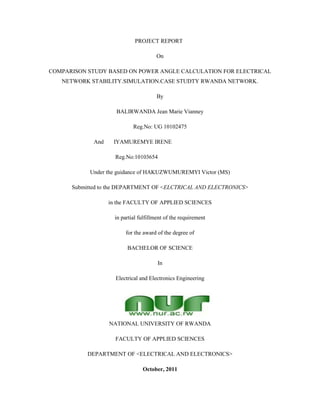
  • 50. 34 3.2.4 Report of the results 3.2.4.1The curve of power transferred and receiving power to the end of the line Figure 3-6 The power angle curve when the reactance x=70mH at the sending end of transmission line. 0 50 100 150 200 250 300 350 400 450 500 0 10 20 30 40 50 60 70 80 90 100110120130140150160170180190 powertransferinwatt Angle in degree
  • 51. 35 Figure 3-7 The power angle curve when the reactance x=70mH at the receiving end of the transmission line. 0 50 100 150 200 250 300 350 400 450 500 0 10 20 30 40 50 60 70 80 90 100110120130140150160170180190 powerreceivedinwatt Angle in degree
  • 52. 36 Figure 3-8 The power angle curve when the reactance x=520mH at the sending end of the transmission line. 0 2 4 6 8 10 12 14 16 18 20 22 24 26 28 30 32 34 36 38 40 42 44 46 48 50 52 54 56 58 60 62 64 66 0 10 20 30 40 50 60 70 80 90 100 110 120 130 140 150 160 170 180 190 powertransferinwatt rotor angle in degree
  • 53. 37 . Figure 3-9 The power angle curve when the reactance x=520mH at the receiving end of transmission line. 0 2 4 6 8 10 12 14 16 18 20 22 24 26 28 30 32 34 36 38 40 42 44 46 48 50 52 54 56 58 60 62 64 66 0 10 20 30 40 50 60 70 80 90 100 110 120 130 140 150 160 170 180 190 powerreceivedinwatt rotor angle in degree
  • 54. 38 3.2.4.2 The steady state stability limit The steady state stability limit is the maximum power that can be transferred by a machine to a receiving system without loss of synchronism, given by the following expression: The steady-state stability limits for the power-angle curve is P transferred=61.24 watt when X=520mH. P transferred =454.95 watt when the X=70mH Comparing the results in two cases with the theoretical value of power transferred to the end of the transmission is almost the same the small change is due to the resistance of the transmission line because in theory the resistance of the line is negligible. 3.2.4.3 The calculation of ∆P/∆V at =30 ,and Vs=Vr=100 The following are the results we have found; ∆P1/∆V=P2-P1/∆V =33.76-30.62/5=0.628 A ∆P2/∆V=P3-P2/∆V=37.05-33.76/5=0.658 A ∆P3/∆V=P4-P3/∆V=40.5-37.05/5=0.69 A ∆P4/∆V=P5-P4/∆V=44.09-40.5/5=0.718 A The value used in calculation are located in the table 3-2.we observe that the ∆P/∆V at fixed angle indicate the variation of current at the same value of the angle.
  • 55. 39 CHAPTER IV: ITERPRETATIONS OF THE RESULTS 4.1 Introduction This chapter will discuss on results that we have got from simulation and calculation. Interpretation of those results will go with the proposed solution for a sustainable stability for electrical network stability based on power angle calculation when the changes in power transfer for variations in transfer reactance and sending end and receiving end voltages are studied in order to plot graph which representing the power angle characteristic for transmission line. 4.2 The discussion made on the results The observation we have seen for the results presented in the table 3-1 is that when we reduce the value of the reactance for the transmission line the current increases in the line and the power transferred at the of the line increases also. The transferred power (sending end power) and the receiving end power to the transmission line are the same considering the lossless line and considering negligible the value of the resistance of the line for all values of the angle. The below figures illustrate that the power transferred to the end of the line and the receiving power for the same value of the reactance of the line are the same for all given angles.
  • 56. 40 Figure 4-1 Power angle curve of sending end and receiving end power of the line x=520mH 0 2 4 6 8 10 12 14 16 18 20 22 24 26 28 30 32 34 36 38 40 42 44 46 48 50 52 54 56 58 60 62 64 66 0 10 20 30 40 50 60 70 80 90 100110120130140150160170180190 powertransferinwatt rotor angle in degree 0 2 4 6 8 10 12 14 16 18 20 22 24 26 28 30 32 34 36 38 40 42 44 46 48 50 52 54 56 58 60 62 64 66 0 10 20 30 40 50 60 70 80 90 100 110 120 130 140 150 160 170 180 190 powerreceivedinwatt rotor angle in degree
  • 57. 41 The steady state stability limit of a particular circuit of a power system is defined as the maximum power that can be transmitted to the receiving end without loss of synchronism; in the above situation is obtained for angle of 90 degree. In steady state the power transferred by synchronous machine is always less than the steady state stability limit. The transient stability limit is the max power that can be transmitted by a machine to a fault or a receiving system during a transient state without loss of synchronism. The transient stability limit is always less than the steady state stability limit. The methods of improving the transient stability limit of a power system.  Reduction in system transfer reactance  Increase of system voltage  Use of high speed excitation systems  Use of high speed reclosing breakers Figure4-2The simulated Data of a short transmission line.
  • 58. 42 During the excitation of the interconnected generators the angle δ cannot change instantaneously due to the inertia of rotating masses. Mechanical power becomes greater than the electric power, hence causing an acceleration of the rotor (i.e., positive acceleration power). As the rotor accelerates, it gains kinetic energy, and the internal angle increases until the electrical power becomes greater than the mechanical power. The rotor decelerates thus releasing the stored kinetic energy gained during the acceleration phase. During this phase, the rotor speed is still higher than the synchronous speed; hence the angle δ continues to increase until the rotor speed is equal to the synchronous speed and δ(rotor angle) = δ2(load angle), the maximum value of the internal angle. But electric power is always greater than the mechanical power. Hence, the rotor will continue to slow and its speed falls below the synchronous speed. The different reading indicate by the displayer at the sending end and receiving end of the transmission line are not exactly the same because of the losses in transmission line due to the resistance of the line that is why the theoretical values are not the same as the simulated value unless when we consider the resistance of the line equal to zero which is not exist in realty.
  • 59. 43 Figure 4-3 Shows the displayer of the scope for the transmitted power for scope displayer 1; the currents on the scope displayer 2 and voltage on the scope displayer 3 in function of time are the same as the receiving end data.
  • 60. 44 CHAPTER V: CONCLUSION AND RECOMMENDATIONS 5.1. CONCLUSION The aim of this project was to study the change in power transfer for variations in transfer reactance and sending end and receiving end voltages, to plot of graph for power angle characteristic is made in order to see for which angle we have maximum power transfer in transmission line in different portions of the Rwanda network; it has been achieved for predicting future planning and operation of the power system. The output of data analysis is the simulation by controlling both rotor angle and power transmitted at the end of the line provide enough information based on which it becomes easy to know the steady state stability limit when we are in interconnected system (synchronous system). To meet rising demand of power, FACTS devices are introduced in the transmission line to enhance its power transfer capability; either in series or in shunt. The series compensations are an economic method of improving power transmission capability of the lines. Thyristor-controlled series capacitors (TCSC) is also a type of series compensator, can provide many benefits for a power system including controlling power flow in the line. In the interconnected network, the purpose is to have an optimum power flow (power transfer to the end of the line) during full service, then to reach a unit power factor which is not practically realizable because of daily variation of inductive loads in the network, for that reason the power factor in the network must be corrected to the value nearby the unit power factor, hence the power angle must be closed to 90 degree.
  • 61. 45 5.2 RECOMMENDATIONS The analysis based simulation of network is a good study for all researchers to be able to predict and forecast the best future state stability of a power system. The researchers in determination of power angle characteristic for a transmission line should be interested in such studies in order to do the modeling and master the operation of electrical networks based on power angle calculations for electrical network stability. Further works should be conducted for whole transmission line of the Rwanda network using advanced and updated software in order to give the general view on power transmitted depending on the expansion of Rwanda network. Other recommendation goes to the National University of Rwanda whereby workshop and practical training on software such as MATLAB, SCADA and POWERWORLD SIMULATOR should be given to students in order to help them feeling more confident and being familiar with software as future Engineers. Recommendation also goes to EWSA which is the company in charge of energy in Rwanda must provide more investment to the students who want to do the reaches on the topics related to the improvement of the sources of energy in our country.
  • 62. 46 REFERENCES Bibliography [1](kundur prabha;”power system stability and control”the EPRI power system Engineering series ISBN: 007035958x). [2] Kundur, P. et al. "Definition and Classification of Power System Stability" IEEE Transactions On Power Systems, 2004, Vol. 19, pp. 1387-1401 [3] Richard G. Farmer "Power System Dynamics and Stability" Taylor & Francis Group, LLC, 2006 [4] Hsu, Yuan-Yih et al. "Identification of optimum location for stabiliser applications using participation factors" IEE Proceedings on Generation, Transmission and Distribution, 1987, Vol. 134, pp. 238-244 [5] Rodriguez, O. et al. "A Comparative Analysis of Methodologies for the Representation of Nonlinear Oscillations in Dynamic Systems" IEEE Lausanne Power Tech, 2007, pp. 172-177 [6] Graham Rogers, “Power System Oscillations”, Kluwer Academic Publishers, USA, 2000. [7] Kundur, P. "Power System Stability and Control" Electric Power Research Institute, McGraw-Hill, Inc. 1994 [8] M .A Pai, Power System Stability New York: North-Holland, 1981 [9] H. Saadat, Power System Analysis McGraw-Hill International Editions, 1999 [10] L. Z. Racz and B. Bokay, Power System Stability Amsterdam; New York: Elsevier, 1988 [11] I. A. Hiskens and D. J. Hills, “Energy Functions, Transient Stability and Voltage
  • 63. 47 Behaviour in Power System with Non-Linear Loads”, IEEE Trans. on Power Systems, Vol 4, No.4, October 1989 [12] P. A Lof and G. Andersson, “Voltage Stability Indices for Stressed Power System”, IEEE Trans. on Power System, Vol 8, No.1, February 1993 [13] Y. Y. Wang, L. Gao, D. J. Hills and R. H. Middleton, “Transient Stability Enhancement and Voltage Regulation of Power System”, IEEE Trans. on Power System, Vol.8, No.2, May 1993 [14] D. J. Hill and I. M. Y. Mareels, “Stability Theory for Differential/ Algebraic Systems with Application to Power System”, IEEE Trans. on Circuit and System, Vol.37, No.11, November 1990 [15] D. J. Hills and I. A. Hiskens, “Dynamic Analysis of Voltage Collapse in Power Systems”, Department of Electrical & Computer Engineering, The University of Newcastle, University Drive, Callaghan, NSW 2308, Australia, December 1992 [16] M. A. Pai, Power System Stability Volume 3: Analysis by the Direct Method of Lyapunov, New York: North-Holland, 1981 [17] Selden B. Crary, Power System Stability Volume 2: Transient Stability, New York: John Wiley & Sons INC, 1962 [18] Allan M. Krall, Stability Techniques for Continuous Linear Systems, Thomas Nelson and Sons Ltd, 1967 [19] Edward Wilson Kimbark, Power System Stability Volume 1: Elements of Stability Calculations, John Wiley & Sons INC, 1957
  • 64. 48 [20] Yi Guo, David J. Hill and Youyi Wang, “Nonlinear decentralized control of large- scale power systems”, Automatica, December 1999 [21] S S Choi, G Shrestha and F Jiang, “Power System Stability Enhancement by Variable Series Compensation”, IPEC 95, Precedings of the International Power Engineering Conference, Vol 1, NTU, Singapore, 27 Feb – 1 Mar 1995 [22] J J Grainger, W D Stevenson, Jr, Power System Analysis, McGraw – Hill, 1994 [23]Abed, A.M., WSCC voltage stability criteria, undervoltage load shedding strategy, and reactive power reserve monitoring methodology, in Proceedings of the 1999 [24] IEEE PES Summer Meeting, Edmonton, Alberta, 191, 1999. [25]Chow, Q.B., Kundur, P., Acchione, P.N., and Lautsch, B., Improving nuclear generating station responsefor electrical grid islanding, IEEE Trans., EC-4, 3, 406, 1989. [26]CIGRE Task Force 38.02.14 report, Analysis and modelling needs of power systems under major frequency disturbances, 1999. [27]CIGRE Working Group 14.05 report, Guide for planning DC links terminating at AC systems locations having short-circuit capacities, Part I: AC=DC Interaction Phenomena, CIGRE GuideNo. 95, 1992. [28]Converti, V., Gelopulos, D.P., Housely, M., and Steinbrenner, G., Long-term stability solution ofinterconnected power systems, IEEE Trans., PAS-95, 1, 96, 1976. [29]Davidson, D.R., Ewart, D.N., and Kirchmayer, L.K., Long term dynamic response of power systems an analysis of major disturbances, IEEE Trans., PAS-94, 819, 1975. [30]EPRI Report EL-6627, Long-term dynamics simulation: Modeling requirements, Final Report of Project 2473-22, Prepared by Ontario Hydro, 1989. [31]Evans, R.D. and Bergvall, R.C., Experimental analysis of stability and power limitations, AIEE Trans.,39, 1924.
  • 65. 49 [32]Gao, B., Morison, G.K., and Kundur, P., Towards the development of a systematic approach for voltage stability assessment of large scale power systems, IEEE Trans. on Power Systems, 11, 3, 1314, 1996. [33]Gao, B., Morison, G.K., and Kundur, P., Voltage stability evaluation using modal analysis, IEEE Trans.PWRS-7, 4, 1529, 1992. [34]IEEE Special Publication 90TH0358-2-PWR, Voltage Stability of Power Systems: Concepts, Analytical Tools and Industry Experience, 1990. Webgraphy [35]http://web.princeton.edu/sites/ehs/labsafetymanual/sec7g.htm [36] http://www.ifp.illinois.edu/~zzhao/ece563/handouts/verdu.pdf [37]http://books.google.rw/books?id=Su3-0UhVF28C&pg=PA537&lpg=PA537&dq
  • 66. I APPENDIX 1 angle Sine angle 0 0 10 0.174 20 0.342 30 0.5 40 0.643 50 0.766 60 0.866 70 0.940 80 0.985 90 1 100 0.985 110 0.940 120 0.866 130 0.766 140 0.643 150 0.5 160 0.342 170 0.174 180 0 This table shows the relation between a given angle and its sine
  • 67. II APPENDIX 2 The displayed values for the following figures for the power must be multiplied by the sine of the corresponding sine angle value. The following values are displayed from 150-180 degrees