1. 1.2.1. Introduction
Divide-and-conquer is a top-down technique for designing algorithms that
consists of dividing the problem into smaller sub problems hoping that the solutions
of the sub problems are easier to find and then composing the partial solutions into
the solution of the original problem.
1. Divide: Break the problem into sub-problems of same type.
2. Conquer: Recursively solve these sub-problems.
3. Combine: Combine the solution sub-problems
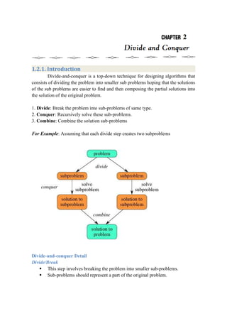
For Example: Assuming that each divide step creates two subproblems
Divide-and-conquer Detail
Divide/Break
This step involves breaking the problem into smaller sub-problems.
Sub-problems should represent a part of the original problem.
2. This step generally takes a recursive approach to divide the problem until
no sub-problem is further divisible.
At this stage, sub-problems become atomic in nature but still represent
some part of the actual problem.
Conquer/Solve
This step receives a lot of smaller subproblems to be solved.
Generally, at this level, the problems are considered 'solved' on their own.
Merge/Combine
When the smaller sub-problems are solved, this stage recursively combines
them until they formulate a solution of the original problem.
This algorithmic approach works recursively and conquer & merge steps
works so close that they appear as one.
Advantages of D & C
1. Solving difficult problems:
Divide and conquer is a powerful tool for solving conceptually difficult
problems: all it requires is a way of breaking the problem into sub-problems, of
solving the trivial cases and of combining subproblems to the original problem.
2. Parallelism:
Divide and conquer algorithms are naturally adapted for execution in multi-
processor machines, especially shared-memory systems where the communication
of data between processors does not need to be planned in advance, because distinct
sub-problems can be executed on different processors.
3. Memory Access:
Divide-and-conquer algorithms naturally tend to make efficient use of
memory caches. The reason is that once a sub-problem is small enough, it and all its
sub-problems can, in principle, be solved within the cache, without accessing the
slower main memory.
4. Roundoff control:
In computations with rounded arithmetic, e.g. with floating point numbers,
a divide-and-conquer algorithm may yield more accurate results than a superficially
equivalent iterative method.
Advantages of D & C
1. For solving difficult problems like Tower Of Hanoi, divide & conquer is a
powerful tool
2. Results in efficient algorithms.
3. 3. Divide & Conquer algorithms are adapted foe execution in multi-processor
machines
4. Results in algorithms that use memory cache efficiently.
Limitations of D & C
1. Recursion is slow.
2. Very simple problem may be more complicated than an iterative approach.
Example: adding n numbers etc
Algorithm
algorithm dc(p)
{
if p is too small then
return solution of p.
else
{
divide (P) and obtain P1,P2,…Pn
where n>=1
apply DC to each subproblem
return combine (DC(P1),DC(P2)..(DC(Pn));
}
}
Recurrence
If we want to divide a problem of size n into a size of n/b taking f(n) time
to divide and combine, then we can set up recurrence relation for obtaining time for
size n is –
The initial recursive equation for T(n) can be drawn with the combine cost as the
root and the recursive pieces as the leaves as
4. Expanding the recursive terms using n/2 gives
Finally we continue to expand the recursive terms until n=1 (giving n leaves at the
last level).
5. The above equation is called general divide and conquer recurrence. The order of
growth of T(n) depends upon the constants a,b and order of growth function f(n).
1.2.2. The substitution method for solving recurrences
The substitution method is kind of method in which a guess for the solution
is made
There are two types of substitution
Forward substitution
Backward substitution
Forward substitution method: this method makes use of an initial condition in the
initial term and value for the next term is generated. This process is continued until
some formula is guessed. Thus in this kind of substitution method,we use
recurrence equation to generate the few terms.
6. For example:
Consider a recurrence relation
T (n) = T (n-1) + n
With initial condition T (0) = 0.
Let,
T (n) = T (n-1) + n
If n = 1 then T (1) = T (1-1) +1 T (0) + 1 0+1 1
If n = 2 then T (2) = T (2-1) +1 T (1) + 2 1+2 3
If n = 3 then T (3) = T (3-1) +3 T (2) + 3 3+3 6
By observing above generated equations we can derive a formula
we can also denote T(n) in terms of big oh notation as follows –
T(n) = O (n2
)
But in practice, it is difficult to guess the pattern from forward
substitution. Hence this method in not very often used.
Backward substitution method: in this method backward values are substituted
recursively in order to derive some formula
For example
Consider, a recurrence relation
T (n) = T (n-1) + n …….. (1)
With initial condition T (0) = 0.
T (n - 1) = T (n-1 -1) + (n – 1) …….. (2)
Putting equation (2) in equation (1) we get,
T (n) = T (n -2 ) + (n – 1) + n ….. (3)
Let
T (n - 2) = T (n-2 -1) + (n – 2) ………(4)
Putting equation (4) in equation (3) we get,
T (n) = T (n -3 ) + (n – 2) + (n – 1) + n
7. T(n) = T (n – k) + ( n – k + 1 ) + ( n – k + 2 ) +…+ n
If k = n then
T (n) = T (0) + 1 + 2 +…n
T (n) = 0 + 1 + 2 +…n
Again
we can also denote T(n) in terms of big oh notation as follows –
T(n) = O (n2
)
1.2.3. Maximum Sub Array Problem
Formal Problem Definition
Given a sequence of numbers <a1,a2,…..an> we work to find a
subsequence of A that is contiguous and whose values have the maximum sum.
Maximum Subarray problem is only challenging when having both positive
and negative numbers.
Example…
Here, the subarray A[8…11] is the Maximum Subarray, with sum 43, has
the greatest sum of any contiguous subarray of array A.
We take an array A
We divide it into two halfes
Maximum subarray in left half is from A1 to A4 with total sum 5
8. Maximum subarray in right half is from A9 to A11 with total sum 25
Maximum subarray at midpoint is from A8 to A11 with total sum 43
The subarray from A8 to A11 has the largest sum and we take it as
maximum subarray.
Brute Force Solution
To solve the Maximum Subarray Problem we can use brute force solution
however in brute force we will have to compare all possible continuous subarray
which will increase running time. Brute force will result in (n2), and the best weѲ
can hope for is to evaluate each pair in constant time which will result in (n2).Ὠ
Divide and Conquer is a more efficient method for solving large number of
problems resulting in (nlogn).Ѳ
Divide and Conquer Solution
First we Divide the array A [low … high] into two subarrays A [low …
mid] (left) and A [mid +1 … high] (right).
We recursively find the maximum subarray of A [low … mid] (left), and
the maximum of A [mid +1 … high] (right).
We also find maximum crossing subarray that crosses the midpoint.
Finally we take a subarray with the largest sum out of three.
Time Analysis
Find-Max-Cross-Subarray takes: (n) timeѲ
Two recursive calls on input size n/2 takes: 2T(n/2) time
Hence:
T(n) = 2T(n/2) + (n)Ѳ
T(n) = (n log n)Ѳ
9. Pseudo Code
Max-subarray(A, Left, Right)
if (Right == Left)
return (left, right, A[left])
else mid= [(left+right)/2]
L1=Find-Maximum-Subarray(A,left,mid)
R1=Find-Maximum-Subarray(A,mid+1,right)
M1=Find-Max-Crossing-Subarray(A,left,mid,right)
If sum(L1) > sum(R1) and sum(L1) > sum(M1)
Return L1
elseif sum(R1) > sum(L1) and sum(R1) > sum(M1)
Return R1
Else return M1
1.2.4. Strassen’s Matrix Multiplication
The Strassen’s Matrix Multiplication find the product C of two 2 × 2
matrices A and B with just seven multiplications as opposed to the eight required by
the brute-force algorithm.
where
Thus, to multiply two 2 × 2 matrices, Strassen’s algorithm makes 7
multiplications and 18 additions/subtractions, whereas the brute-force algorithm
requires 8 multiplications and 4 additions. These numbers should not lead us to
multiplying 2 × 2 matrices by Strassen’s algorithm. Its
importance stems from its asymptotic superiority as matrix order n goes to infinity.
10. Let A and B be two n × n matrices where n is a power of 2. (If n is not a
power of 2, matrices can be padded with rows and columns of zeros.) We can divide
A, B, and their product C into four n/2 × n/2 submatrices each as follows:
The value C00 can be computed either as A00 * B00 + A01 * B10 or as M1 +
M4 − M5 + M7 where M1, M4, M5, and M7 are found by Strassen’s formulas, with
the numbers replaced by the corresponding submatrices. The seven products of n/2
× n/2 matrices are computed recursively by Strassen’s matrix multiplication
algorithm.
The asymptotic efficiency of Strassen’s matrix multiplication algorithm
If M(n) is the number of multiplications made by Strassen’s algorithm in
multiplying two n×n matrices, where n is a power of 2, The recurrence relation is
M(n) = 7M(n/2) for n > 1, M(1)=1.
Since n = 2k
,
M(2k
) = 7M(2k−1
)
7[7M(2k−2
)]
72
M(2k−2
)
. . .
7i
M(2k−i
)
. . .
= 7k
M(2k−k
) = 7k
M(20
) = 7k
M(1) = 7k
(1)
(Since M(1)=1)
M(2k
) = 7k
.
Since k = log2 n,
= 7log n
M(n) 2
= log 7
n 2
n2.807
Which is smaller than n3
required by the brute-force algorithm.
11. Since this savings in the number of multiplications was achieved at the
expense of making extra additions, we must check the number of additions A(n)
made by Strassen’s algorithm. To multiply two matrices of order n>1, the algorithm
needs to multiply seven matrices of order n/2 and make 18 additions/subtractions of
matrices of size n/2; when n = 1, no additions are made since two numbers are
simply multiplied. These observations yield the following recurrence relation:
12. 1.2.5. The Recursion Tree Method for solving recurrences
In a recursion tree ,each node represents the cost of a single sub-problem
somewhere in the set of recursive problems invocations .we sum the cost within
each level of the tree to obtain a set of per level cost, and then we sum all the per
level cost to determine the total cost of all levels of recursion.
A recursion tree can be used to visualize the iteration procedure. The idea
of a Recursion tree is to expand T (n) to a tree with the same total cost.
Important points:
The height of the tree
The cost of the nodes at each level
Sum up the costs of all levels.
Ex:-
13. 1.2.6. The Master method for solving recurrences
A utility method for analyzing recurrence relations
Useful in many cases for divide and conquer algorithms.
These recurrence relations are of the form
a>=1, b>1
n = the size of current problem
a = no. of sub problems in the recursion
n/b = the size of each sub problem
f(n) = the cost of the work that has to be done outside.
The recursive calls (cost of dividing + merging)
There are 3 cases:
Case 1. The running time is dominated by the cost at the levels.
If , then for .
Case 2. The running time is dominated by the cost at the root.
If , then for an E>0.
If f (n) satisfies the regularity condition:
14. Where c<1
(this always holds for polynomials). Because of this condition, the
master method cannot solve every recurrence of the given form.
Case 3.The running time is evenly distributed throughout the tree.
If , then .
How to apply the master method (Step-by-step)?
1. Extract a, b and f (n) from a given recurrence
2. Determine .
3. Compare f (n) and asymptotically.
4. Determine the appropriate master method case and apply it.
Example 1:
Imagine that
1. Extract; a = 2, b = 2 and f (n) = n
2. Determine;
3. Compare; f (n) = n
4. Thus case 3; evenly distributed because .
.
Example 2:
Imagine that
1. Extract; a = 9, b = 3, f (n) = n
2. Determine;
15. 3. Compare; f (n) = n
∴ n<n2
4. Thus case 1 express f (n) in terms of
Example 3:
Imagine that
1. Extract; a = 3, b = 4, f (n) = n log(n)
2. Determine; where
3. Compare;
4. Thus case 2; but we have to check the regularity condition 1.
The following should be true
Where c<1
This true for c = ¾.
For example,
So Because