Design and Analysis of Algorithms

1. 4.1.1. Introduction
Graphs are mathematical structures that represent pairwise relationships
between objects. A graph is a flow structure that represents the relationship between
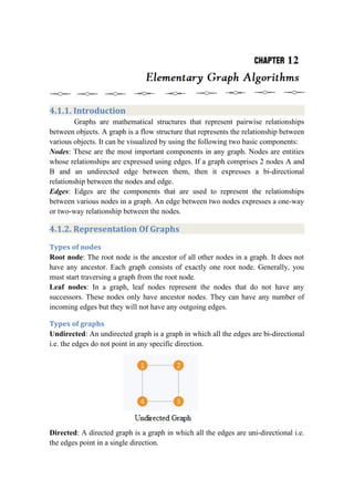
various objects. It can be visualized by using the following two basic components:
Nodes: These are the most important components in any graph. Nodes are entities
whose relationships are expressed using edges. If a graph comprises 2 nodes A and
B and an undirected edge between them, then it expresses a bi-directional
relationship between the nodes and edge.
Edges: Edges are the components that are used to represent the relationships
between various nodes in a graph. An edge between two nodes expresses a one-way
or two-way relationship between the nodes.
4.1.2. Representation Of Graphs
Types of nodes
Root node: The root node is the ancestor of all other nodes in a graph. It does not
have any ancestor. Each graph consists of exactly one root node. Generally, you
must start traversing a graph from the root node.
Leaf nodes: In a graph, leaf nodes represent the nodes that do not have any
successors. These nodes only have ancestor nodes. They can have any number of
incoming edges but they will not have any outgoing edges.
Types of graphs
Undirected: An undirected graph is a graph in which all the edges are bi-directional
i.e. the edges do not point in any specific direction.
Directed: A directed graph is a graph in which all the edges are uni-directional i.e.
the edges point in a single direction.

2. Weighted: In a weighted graph, each edge is assigned a weight or cost. Consider a
graph of 4 nodes as in the diagram below. As you can see each edge has a
weight/cost assigned to it. If you want to go from vertex 1 to vertex 3, you can take
one of the following 3 paths:
1 -> 2 -> 3
1 -> 3
1 -> 4 -> 3
Therefore the total cost of each path will be as follows: - The total cost of 1 -> 2 ->
3 will be (1 + 2) i.e. 3 units - The total cost of 1 -> 3 will be 1 unit - The total cost
of 1 -> 4 -> 3 will be (3 + 2) i.e. 5 units
Cyclic: A graph is cyclic if the graph comprises a path that starts from a vertex and
ends at the same vertex. That path is called a cycle. An acyclic graph is a graph that
has no cycle.
A tree is an undirected graph in which any two vertices are connected by only one
path. A tree is an acyclic graph and has N - 1 edges where N is the number of
vertices. Each node in a graph may have one or multiple parent nodes. However, in
a tree, each node (except the root node) comprises exactly one parent node.

3. Note: A root node has no parent.
A tree cannot contain any cycles or self loops, however, the same does not apply to
graphs.
Graph representation
You can represent a graph in many ways. The two most common ways of
representing a graph is as follows:
Adjacency matrix
An adjacency matrix is a VxV binary matrix A. Element Ai,j is 1 if there is
an edge from vertex i to vertex j else Ai,j is 0.
Note: A binary matrix is a matrix in which the cells can have only one of two
possible values - either a 0 or 1.
The adjacency matrix can also be modified for the weighted graph in which instead
of storing 0 or 1 in Ai,j, the weight or cost of the edge will be stored.
In an undirected graph, if Ai,j = 1, then Aj,i = 1. In a directed graph, if Ai,j
= 1, then Aj,i may or may not be 1.
Adjacency matrix provides constant time access (O(1) ) to determine if
there is an edge between two nodes. Space complexity of the adjacency matrix is
O(V2).
The adjacency matrix of the following graph is:

4. The adjacency matrix of the following graph is:
Consider the directed graph given above. Let's create this graph using an adjacency
matrix and then show all the edges that exist in the graph.
Input file
4 // nodes
5 //edges
1 2 //showing edge from node 1 to node 2
2 4 //showing edge from node 2 to node 4
3 1 //showing edge from node 3 to node 1
3 4 //showing edge from node 3 to node 4
4 2 //showing edge from node 4 to node 2
Adjacency list
The other way to represent a graph is by using an adjacency list. An
adjacency list is an array A of separate lists. Each element of the array Ai is a list,
which contains all the vertices that are adjacent to vertex i.
For a weighted graph, the weight or cost of the edge is stored along with the
vertex in the list using pairs. In an undirected graph, if vertex j is in list Ai then
vertex i will be in list Aj.

5. The space complexity of adjacency list is O(V + E) because in an adjacency
list information is stored only for those edges that actually exist in the graph. In a lot
of cases, where a matrix is sparse using an adjacency matrix may not be very useful.
This is because using an adjacency matrix will take up a lot of space where most of
the elements will be 0, anyway. In such cases, using an adjacency list is better.
Note: A sparse matrix is a matrix in which most of the elements are zero, whereas a
dense matrix is a matrix in which most of the elements are non-zero.
A1 → 2 → 4
A2 → 1 → 3
A3 → 2 → 4
A4 → 1 → 3
Consider the same undirected graph from an adjacency matrix. The adjacency list of
the graph is as follows
Consider the same directed graph from an adjacency matrix. The adjacency list of
the graph is as follows:
A1 → 2
A2 → 4
A3 → 1 → 4
A4 → 2

6. Consider the directed graph given above. The code for this graph is as follows:
Input file
4 // nodes
5 //edges
1 2 //showing edge from node 1 to node 2
2 4 //showing edge from node 2 to node 4
3 1 //showing edge from node 3 to node 1
3 4 //showing edge from node 3 to node 4
4 2 //showing edge from node 4 to node 2
Graph traversals
Graph traversal means visiting every vertex and edge exactly once in a
well-defined order. While using certain graph algorithms, you must ensure that each
vertex of the graph is visited exactly once. The order in which the vertices are
visited are important and may depend upon the algorithm or question that you are
solving.
During a traversal, it is important that you track which vertices have been
visited. The most common way of tracking vertices is to mark them.
4.1.3. Breadth First Search (BFS)
There are many ways to traverse graphs. BFS is the most commonly used
approach.
BFS is a traversing algorithm where you should start traversing from a
selected node (source or starting node) and traverse the graph layerwise thus
exploring the neighbour nodes (nodes which are directly connected to source node).
You must then move towards the next-level neighbour nodes.
As the name BFS suggests, you are required to traverse the graph
breadthwise as follows:
First move horizontally and visit all the nodes of the current layer
 Move to the next layer
 Consider the following diagram.
Algorithm

8. The traversing will start from the source node and push s in queue. s will be
marked as 'visited'.
First iteration
 s will be popped from the queue
 Neighbors of s i.e. 1 and 2 will be traversed
 1 and 2, which have not been traversed earlier, are traversed. They will be:
o Pushed in the queue
o 1 and 2 will be marked as visited
Second iteration
 1 is popped from the queue

9.  Neighbors of 1 i.e. s and 3 are traversed
 s is ignored because it is marked as 'visited'
 3, which has not been traversed earlier, is traversed. It is:
o Pushed in the queue
o Marked as visited
Third iteration
 2 is popped from the queue
 Neighbors of 2 i.e. s, 3, and 4 are traversed
 3 and s are ignored because they are marked as 'visited'
 4, which has not been traversed earlier, is traversed. It is:
o Pushed in the queue
o Marked as visited
Fourth iteration
 3 is popped from the queue
 Neighbors of 3 i.e. 1, 2, and 5 are traversed
 1 and 2 are ignored because they are marked as 'visited'
 5, which has not been traversed earlier, is traversed. It is:
o Pushed in the queue
o Marked as visited
Fifth iteration
 4 will be popped from the queue
 Neighbors of 4 i.e. 2 is traversed
 2 is ignored because it is already marked as 'visited'
Sixth iteration
 5 is popped from the queue
 Neighbors of 5 i.e. 3 is traversed
 3 is ignored because it is already marked as 'visited'
The queue is empty and it comes out of the loop. All the nodes have been
traversed by using BFS.
If all the edges in a graph are of the same weight, then BFS can also be used to
find the minimum distance between the nodes in a graph.

10. As in this diagram, start from the source node, to find the distance between
the source node and node 1. If you do not follow the BFS algorithm, you can go
from the source node to node 2 and then to node 1. This approach will calculate the
distance between the source node and node 1 as 2, whereas, the minimum distance
is actually 1. The minimum distance can be calculated correctly by using the BFS
algorithm.
Complexity
The time complexity of BFS is O(V + E), where V is the number of nodes
and E is the number of edges.
4.1.4. Depth First Search (DFS)
The DFS algorithm is a recursive algorithm that uses the idea of
backtracking. It involves exhaustive searches of all the nodes by going ahead, if
possible, else by backtracking.
Here, the word backtrack means that when you are moving forward and
there are no more nodes along the current path, you move backwards on the same
path to find nodes to traverse. All the nodes will be visited on the current path till all
the unvisited nodes have been traversed after which the next path will be selected.
This recursive nature of DFS can be implemented using stacks. The basic
idea is as follows:
Pick a starting node and push all its adjacent nodes into a stack.
Pop a node from stack to select the next node to visit and push all its
adjacent nodes into a stack.
Repeat this process until the stack is empty. However, ensure that the nodes
that are visited are marked. This will prevent you from visiting the same node more
than once. If you do not mark the nodes that are visited and you visit the same node
more than once, you may end up in an infinite loop.

11. Algorithm
The following image shows how DFS works.
Time complexity
Time complexity O(V+E), when implemented using an adjacency list.

12. Applications
How to find connected components using DFS?
A graph is said to be disconnected if it is not connected, i.e. if two nodes
exist in the graph such that there is no edge in between those nodes. In an
undirected graph, a connected component is a set of vertices in a graph that are
linked to each other by paths.
Consider the example given in the diagram. Graph G is a disconnected
graph and has the following 3 connected components.
First connected component is 1 -> 2 -> 3 as they are linked to each other
Second connected component 4 -> 5
Third connected component is vertex 6
In DFS, if we start from a start node it will mark all the nodes connected to
the start node as visited. Therefore, if we choose any node in a connected
component and run DFS on that node it will mark the whole connected component
as visited.

13. 4.1.5. Topological sort
Topological sorting of vertices of a Directed Acyclic Graph is an ordering
of the vertices v1,v2,...vn in such a way, that if there is an edge directed towards
vertex vj from vertex vi, then vi comes before vj.
For example consider the graph given below:
A topological sorting of this graph is: 1 2 3 4 5 There are multiple
topological sorting possible for a graph. For the graph given above one another
topological sorting is: 1 2 3 4 5
In order to have a topological sorting the graph must not contain any cycles.
In order to prove it, let's assume there is a cycle made of the vertices v1,v2,v3…vn
That means there is a directed edge between vi and vi+1 (1≤i<n) and between vn and
v1. So now, if we do topological sorting then vn must come before v1 because of the
directed edge from vn to v1. Clearly, vi+1 will come after vi, because of the directed
from vi to vi+1, that means v1 must come before vn. Well, clearly we've reached a
contradiction, here. So topological sorting can be achieved for only directed and
acyclic graphs.
Le'ts see how we can find a topological sorting in a graph. So basically we
want to find a permutation of the vertices in which for every vertex vi, all the
vertices vj having edges coming out and directed towards vi comes before vi. We'll
maintain an array T that will denote our topological sorting. So, let's say for a graph
having N vertices, we have an array
in_degree[] of size N whose ith element tells the number of vertices which are not
already inserted in T and there is an edge from them incident on vertex numbered i.
We'll append vertices vi to the array T, and when we do that we'll decrease the value
of in_degree[vj] by 1 for every edge from vi to vj. Doing this will mean that we
have inserted one vertex having edge directed towards vj. So at any point we can
insert only those vertices for which the value of in_degree[] is 0.

14. Initially in_degree[0]=0 and T is empty
So, we delete 0 from Queue and append it to T. The vertices directly connected to 0
are 1 and 2 so we decrease their in_degree[] by 1. So, now in_degree[1]=0 and so 1
is pushed in Queue.
Next we delete 1 from Queue and append it to T. Doing this we decrease
in_degree[2] by 1, and now it becomes s pushed into Queue.
So, we continue doing like this, and further iterations looks like as follows:

15. So at last we get our Topological sorting in T : 0 1 2 3 4 5