
Recomendados
Más contenido relacionado
Destacado
Destacado (20)
Jmp10 se quick_guide
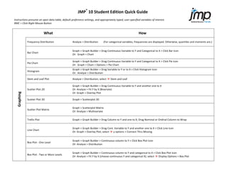
- 1. JMP® 10 Student Edition Quick Guide Instructions presume an open data table, default preference settings, and appropriately typed, user-‐specified variables of interest. RMC = Click Right Mouse Button What How Frequency Distribution Analyze > Distribution (For categorical variables, frequencies are displayed. Otherwise, quantiles and moments are.) Graph > Graph Builder > Drag Continuous Variable to Y and Categorical to X > Click Bar Icon Bar Chart Or: Graph > Chart Graph > Graph Builder > Drag Continuous Variable to Y and Categorical to X > Click Pie Icon Pie Chart Or: Graph > Chart > Options > Pie Chart Graph > Graph Builder > Drag Variable to Y or to X > Click Histogram Icon Histogram Or: Analyze > Distribution Stem and Leaf Plot Analyze > Distribution; select Stem and Leaf Graph > Graph Builder > Drag Continuous Variable to Y and another one to X Scatter Plot 2D Or: Analyze > Fit Y by X (Bivariate) Graphing Or: Graph > Overlay Plot Scatter Plot 3D Graph > Scatterplot 3D Graph > Scatterplot Matrix Scatter Plot Matrix Or: Analyze > Multivariate Trellis Plot Graph > Graph Builder > Drag Column to Y and one to X; Drag Nominal or Ordinal Column to Wrap Graph > Graph Builder > Drag Cont. Variable to Y and another one to X > Click Line Icon Line Chart Or: Graph > Overlay Plot; select y options > Connect Thru Missing Graph > Graph Builder > Continuous column to Y > Click Box Plot Icon Box Plot -‐ One Level Or: Analyze > Distribution Graph > Graph Builder > Continuous column to Y and categorical to X > Click Box Plot Icon Box Plot -‐ Two or More Levels Or: Analyze > Fit Y by X (choose continuous Y and categorical X); select Display Options > Box Plot
- 2. Analyze > Distribution; (basic stats are shown by default; to see more select Display Options) Descriptive statistics or Tables > Summary or Tables > Tabulate 1-‐Sample: Analyze > Distribution; select Test Mean z-‐ or t-‐ test 2-‐Sample: Analyze > Fit Y by X (cont. Y and 2-‐level cat. X); select t Test or Means/ANOVA/Pooled t Basic Statistics Paired t: Analyze > Matched Pairs Testing Proportions (make 0/1 1 Proportion: Analyze > Distribution; select Test Probabilities indicator Nominal or Ordinal) 2 Proportions: Analyze > Fit Y by X Contingency table – Chi-‐Square test Analyze > Fit Y by X (both X and Y must be categorical) Covariance Analyze > Multivariate Methods > Multivariate; select Covariance matrix Analyze > Multivariate Methods > Multivariate Correlation Or Analyze > Fit Y by X > Density Ellipse Test for Normality/Goodness-‐of-‐fit Analyze > Distribution; select Continuous Fit > Normal; select by Fitted Normal > Goodness of Fit On data table: 1. Select Columns > New Column; 2. RMC on new column > Formula; Probability Variables 3. Select Probability from Functions Window; Random Variables 4. Select desired probability function. Probability & Note: For more information on the expected parameters see Help under Probability Functions On data table: On data table: 1. Select Columns > New Column; 1. Select Columns > New Column; 2. RMC on new column > Column Info; or 2. RMC on new column > Formula; Select Random Variables 3. Click on drop down box next to Random from Functions Window; Initialize Data > Random 3. Select desired Random function. Note: For more information on the expected parameters see help under Random Function Distribution Fitting Analyze > Distribution; select Continuous Fit, then select desired distribution(s).
- 3. One-‐Way Analyze > Fit Y by X; select Means/Anova (Y must be continuous; X categorical) Analysis of Variance Two or more Factors Analyze > Fit Model Randomized Blocks Analyze > Fit Y by X; include a categorical column in Block role Multiple Comparison Methods Analyze > Fit Y by X; select Means/Anova; select Compare Means Test for Equal/Unequal Variances Analyze > Fit Y by X; select Means/Anova; select Unequal Variances Analyze > Fit Y by X (Bivariate) Scatter Plot Or, Graph > Graph Builder > Drag continuous column to Y and another to X One Variable: Analyze > Fit continuous Y by continuous X; select Fit Line Simple Least Squares Or, Click Line Icon from Scatterplot in Graph Builder (see above). One or More Independent Variables: Analyze > Fit Model Regression One Variable: Analyze > Fit categorical Y by continuous X Logistic Regression One or more independent variables: Analyze > Fit Model Multiple Regression Analyze > Fit Model Stepwise Regression Analyze > Fit Model > Personality – Select Stepwise Analyze > Fit Model; Run Model; select Row Diagnostics Residual Analysis Or Analyze > Fit Y by X; Select and choose a fit; Select from fit report and “Save Residuals” or “Plot residuals” Interaction Plots Analyze > Fit Model with interaction effects; Run Model; select Factor Profiling > Interaction Plots Durbin-‐Watson Test Analyze > Fit Model; Run; select Row Diagnostics > Durban Watson Test Wilcoxon Rank Sum Test Analyze > Fit Y by X; select Nonparametric > Wilcoxon Test Nonparametric techniques Fishers Sign Test (for 2x2 tables only) Analyze > Fit categorical Y by categorical X Wilcoxon Signed Rank Sum Test Analyze > Distribution on continuous X; select Test Mean > Check Wilcoxon Signed Rank Box Kruskal-‐Wallis Test Analyze > Fit continuous Y by categorical X; select Nonparametric > Wilcoxon Test Spearman’s ρ Analyze > Multivariate; select Nonparametric Correlations > Spearman’s ρ
- 4. Time Series Plot Analyze > Time Series Series Time Moving Averages Analyze > Time Series; select Smoothing Model > Simple Moving Average Exponential Smoothing Analyze > Time Series; select Smoothing Model Holt-‐Winters Method Analyze > Time Series; select Smoothing Model > Winters Method Run Chart: Graph > Control Chart > Run Chart X-‐bar: Graph > Control Chart > Control Chart > XBar Individual Measurements (IR): Graph > Control Chart > Control Chart > IR Quality Control Control Charts P Chart: Graph > Control Chart > Control Chart > P U Chart: Graph > Control Chart > Control Chart > U CUSUM: Graph > Control Chart > Control Chart > CUSUM Pareto Graph > Pareto Plot Capability Graph > Control Chart > IR; check Capability Box. > OK, Fill in Specification Limits DOE > Full Factorial Design Experiments Factorial Design Design Of Or: DOE > Screening Design Screening Design DOE > Screening Design Response Surface Design DOE > Response Surface Design Sample Size and Power Calculations DOE > Sample Size and Power http://www.jmp.com/academic For complete information and tutorials, please refer to the JMP Help available under “Help > Books” and “Help > Tutorials”.