BVQ is the most sophisticated and comprehensive performance and capacity monitoring and performance analysis software in the market for IBM’s storage products IBM SAN Volume Controller (SVC), IBM Storwize V7000 and the new IBM Storwize V3700.

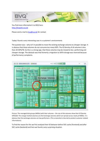
1. You find more information’s to BVQ here:
http://bvqwiki.sva.de
Please send a mail to bvq@sva.de for contact
Today I found a very interesting case in a customer’s environments
The question was – why isn’t it possible to move the existing exchange volumes to cheaper storage. It
is obvious that these volumes do not consume too many IOPS. The IO Density of all volumes is less
than 20 IOPS/TB. So this is a strong sign, that these volumes may be moved to less performing and
cheaper storage. The obstacle was that formerly a migration to SATA storage was reversed because
of performance complaints.
Picture: The managed disk groups (MDGs) with their volumes – the size of the volumes show their IO Denstiy
IOPS/GB. The orange marked volumes are the Exchange volumes which are spread across nearly all MDGs. It is
obvious that the exchange volumes are low performers. (This screenshot is blurred to protect customer related
informations)
To find the reason for this we first analyzed their IO behavior before SVC cache (frontend) and after
SVC cache (backend) and here we found a very surprising situation.

2. The backend IO rate was much higher than the frontend IO rate which is not normal because the SVC
Cache should rather reduce the backedend IORate compared to frontend.
Picture: A very surprising result for the first view – the backend IO Rate is much higher than the
frontend IO Rate. The disks need more than 10000 IOPS in backend so this looks is not very suitable
for slow performing storage
The reason for these high backend storage rate is Thin Provisioning. The volumes has very big
transfer sizes in the front end of sometimes more than 700kb. Thin Provisioning works on grain size
when it sends the data to disk. For this SVC has to break down these big frontend transfer sizes into
32kb backend transfers sizes packages which multiplied the IO rate by factor 3 in mean.
We found this when we analyzed all Volumes in the MDG. One of the volumes had an incredible
backend IO rate which was more than 10 times the frontend IO rate – we saw that the transfer size
was also 10 times the transfer size of the backend. And the backend size was 32kb – grain size – bingo
– thin provisioning.

3. Picture: All Exchange volumes with backend IO rate, Cache size and response time in one chart,. One of the
volumes showed an extremely high backend IO rate with a very big transfers size – we found that the transfer
size of the backend is only a 1/10 of the frontend transfer size and it is exactly the grain size which leads to thin
provisioning.
Last check – where to spare money – Thin Provisioning or cheaper storage or both?
Is Thin Provisioning an economical right decision for these volumes?
We analyzed space efficiency of the volumes an found that the customer has only a win of 3.5% with
the thin provisioning switched on. Thin Provisioning shows 14.3% but there is already allocated o lot
of overhead free memory in the volumes so real saving is only 3.5%.

4. Picture: BVQ Treemap with Volume Groups and Volumes. The space efficiency coloring of the Treemap shows
that Thin Provisioning is not at all effective for all Exchange Volumes. The color Red means that space efficiency
with Thin Provisioning is low. Yellow is more effective - green and blue is very effective – grey shows that no
thins provisioning is in use for these volumes.
Final check to find the correct sizing for the new Exchange disks.
We can assume that SVC will no longer increase the backend transfer size when we switch of Thin Provisioning
for the exchange volumes. So we analyze the frontend portion of the IO and find the following sizing
parameters. With this knowledge we can very exactly determine the minimum sizing for the new disk structure
to host all Exchange volumes. The resul was – taking all caching results + IOPS needs into account we will be
able to cover the workload with only 48 1TB/7.2k disks .
IOPS RW maximum is 3000 IOPS
Worst RW Distribution is 55% Read in maximum of IOPS
Cache hit read is 90%
Cache hit write (overwrite in cache) is aprox 10%

5. +
Picture: Frontend analysis of all exchange volumes to find the correct sizing parameters. 3000 IOPS, 55% RW
Distribution in worst case, 90% cache hit read and 10 % cache hit write (overwrite in cache)