With screenshots, this handout walks the user through an introduction to Excel, including sorting, filtering, functions and pivot tables. It was prepared by Steve Doig, professor of journalism, specializing in data reporting, at the Walter Cronkite School of Journalism and Mass Communication at Arizona State University. He created it for Seattle NewsTrain on Nov. 11, 2017. It accompanies his presentation, Data-Driven Enterprise off Your Beat. NewsTrain is a training initiative of Associated Press Media Editors (APME). More info: http://bit.ly/NewsTrain

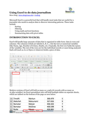
1. Using Excel to do data journalism
Steve Doig | steve.doig@asu.edu | @sdoig
Microsoft Excel is a powerful tool that will handle most tasks that are useful for a
journalist who needs to analyze data to discover interesting patterns. These tasks
include:
 Sorting
 Filtering
 Using math and text functions
 Summarizing data with pivot tables
INTRODUCTION TO EXCEL
Excel will handle large amounts of data that is organized in table form: data in rows and
columns. The columns (which are labeled A, B, C…) list the text or numerical variables
(like Name, Age, Number of Crimes, Deaths, etc.) Typically, the first row holds the names
of the variables. The rest of the rows are for the individual records or cases being analyzed.
Each cell (such as A1 or D502 or whatever) holds a piece of data.
Modern versions of Excel will hold as many as 1,048,576 records with as many as
16,384 variables! An Excel spreadsheet also will hold multiple tables on separate sheets,
which are tabbed on the bottom of the page as seen below:

2. SORTING
One of the most useful abilities of Excel is to sort the data into a more revealing order. Too
often, we are given lists that are in alphabetical order, which is useful only for finding a
particular record in a long list. In journalism, we usually are more interested in extremes:
the most, the least, the biggest, the smallest, the best, the worst.
Consider the data used in this tutorial, a list of the regions and provinces of the mythical
country of Datamania showing the number of various kinds of crimes reported during a
recent year. Here is how it looks sorted in alphabetical order of province name:
Far more interesting would be to sort it in descending order of the total number of
murders, with the murder-plagued province of Makinen at the top of the list:

3. There are two methods of sorting. The first method is quick and can be used for sorting by
a single variable. Just put the cursor in the column you wish to sort by (“murders” in
this case) and then click the Z-to‐A button:
But beware! Put the cursor IN the column, but DO NOT select the whole column by
clicking on the letter (D, in this case) before you sort. Consider the example below:
Doing that will sort ONLY the data in that column, thereby disordering your data! The
province of Aisch had only 8 murders, but as you see below now has 69. Don't make this
mistake!

4. Depending on your version of Excel, you may get a cryptic warning about there being
other data next to it, but some versions of Excel don't give a warning at all. So be
careful.
The other method of sorting is for when you want to sort by more than one variable at a
time. For instance, suppose we wish to sort the crime data first by Region in alphabetical
order, but then sort by “murder” in descending order within each Region. To do that, go to
the toolbar, click on “Data” and then “Sort…”, and then choose the variables by which you
wish to sort. Then click “OK”.
The result will be this:
See how the provinces of Abdullah are listed in descending order of the number of
murders, followed by the Abela provinces, and so on.

5. FILTERING
Sometimes you want to examine only particular records from a large collection of data.
For that, you can use Excel’s Filter tool. On the toolbar, go to “Data…Filter” and the
Autofilter buttons will appear at the top of each column:
Suppose we wish to see the records from only the Rutte region. Click on the button on the
Region column, uncheck "Select All", then scroll down to Rutte on the list and check it.
This is the result:
Notice that you now are seeing only rows 14, 32, 35, etc. Also notice at the very bottom
that Excel tells you " 9 of 103 records found" meeting your condition.

6. More complicated filters are possible. For instance, suppose you wish to see only records in
which the population is greater than or equal to 1,000,000 AND the number of murders is
less than or equal to 20. Fill out the two filters like this:
Here is your result:

7. FUNCTIONS
Excel has many built-in functions useful for performing math calculations and working
with dates and text. For instance, assume that you want to add up the total number of
murders in all of Datamania. To do this, we would go to the bottom of Column D, skip a
row and then enter this formula in Cell C106: =SUM(D2:D104). The equals sign (=) is
necessary for all functions. The colon (:) means “all the numbers from Cell C2 to Cell
104”. The result is this:
(The reason for skipping a row is to separate the sum from the main table so that the table
can be sorted without pulling the sum into the table during the sorting operation. This way
the sum will stay at the bottom of the column.)
Often you will want to do a calculation on each row of your data table. For instance, you
might want to calculate the murder rate (the number of murders per 100,000 population),
which would let you compare the crime problem in cities of different sizes. To do this, we
would create a new variable called “Murder Rate” in Column H, the first empty column.
Then, in Cell H2, we would enter this formula: =(D2/C2)*100000. This divides the
murders by the population, then multiplies the result by 100,000. (Notice that there are
no spaces and no thousands separators used in the formula.) Here is the result:
1,9 is the
European way
of expressing
1.9 in the U.S.

8. It would be very tedious to repeat writing that calculation in each of 103 rows of data.
Happily, Excel has a way to rapidly copy a formula down a column of cells. To do that, you
careful move the cursor (normally a big fat white cross) to the blue button on the
bottom right corner of the cell containing the formula.
When it is in the right spot, the cursor will change to a small black cross. At that point, you
can double-click and the formula will copy down the column until it reaches a blank cell
in the column to the left. This would be the result:
Notice that the formula changes for each row, so that the formula in Row 6 is
=(D6/C6)*100000.
Now, if we sort by Murder Rate in descending order, we see the provinces with the worst
violent crime problems, with the province of Warden in the Merkel region being by far
the worst. Even though the province of Makinen has the most murders (69), it's also the
most populous province, so its murder rate of 2.3 per 100,000 population isn't the worst.
Warden has a much bigger murder problem for its size:

9. Here are a few other useful Excel functions that can be used in similar ways:
• Simple math: Add, subtract, multiply or divide by using the symbols + - * /
• =AVERAGE – calculates the arithmetic mean of a column or row of numbers
• =MEDIAN – finds the middle value of a column or row of numbers
• =COUNT – tells you how many items there are in a column or row
• =MAX – tells you the largest value in a column or row
• =MIN – tells you the smallest value in a column or row
There are also a variety of text functions that can join or cut apart text strings. For instance:
If “Steve” is in Cell B2 and “Doig” is in Cell C2, then =B2&” “&C2 will produce “Steve
Doig”. And
=C2&”, “&B2 will produce “Doig, Steve”. Other useful text functions include:
• =SEARCH – this will find the start of a desired string of text in a larger string.
• =LEN – this will tell you how many characters are in a text string.
• =LEFT – this will extract however many characters you specify starting from the left.
• =RIGHT – this will extract characters starting from the right.
• =MID – this will extract however many characters you specify starting at whatever
point you specify
You can also do date arithmetic, such as calculating the number of days or years between
two dates, or the hours, minutes and seconds between two times. For instance, to calculate
on April 24, 2014, the age in years of someone whose birth date is in cell B2, you could use
this formula:
=(DATE(2014,4,24)-B2)/365.25. The first part of the formula calculates the number of
days
between the two dates, which then is divided by 362.25 (the 0.25 accounts for leap years)
to produce the years. Another useful date function is =WEEKDAY, which will tell you on
which day of the week a chosen date falls. For instance:
=WEEKDAY(DATE(1948,4,21)) returns a 4, which means I was born on a Wednesday.
Excel offers well over 200 functions in a variety of categories beyond just math, dates and
text: financial, engineering, database, logical, statistical, etc. But it is unlikely that you will
need to be familiar with more than a dozen or so functions, unless you are a journalist with
a very specialized beat such as economics.
PIVOT TABLES
One of Excel’s best tricks is the ability to summarize data that is in categories. The tool
that does this is called a pivot table, which creates an interactive cross-tabulation of the
data by category.
To create a pivot table, every column of your data must have a variable label; in fact, it is
always good practice to put in a variable label any time you insert or add a new column.
First, you make sure your cursor is on any one cell in the table. Then go to the tool bar
and click on “Data…Pivot Table...”. A window will pop up labeled “Create Pivot Table ”.
Just hit “OK”.

10. This will open a new worksheet that looks like this:
Notice the elements of the Pivot Table Builder. Your variables are listed under Field Name,
and there are four boxes in which to drag-and-drop variables to make the pivot table.
To build a pivot table, you should visualize the piece of paper that would answer your
question. Our example data shows 103 provinces in the 18 regions of Datamania. Imagine
that you wanted to know the total number of murders in each region. The piece of paper
that would answer that question would be a table that lists each region, with the total
number of murders next to each name.
To build this pivot table, we would use the mouse to pick up “Region” from the list of
variables in the floating box to the right, and place it in the “Row Labels” box. We would
then take the “murders” variable and put it in the “Values” box. This would be the result:

11. If you click the cursor into the “Total” Column and hit the Z<->A button to sort, you will
get this:
You can add other variables to the Values box, such as sum of population:
It is possible to make very complicated pivot tables, with multiple variables and subtotals.
But I recommend making a new pivot table for each question you want to answer; several
simple tables are easier to understand than one very complicated table that tries to answer
many questions at once.

12. You can also make true cross-tabulations with pivot tables. Consider this data from the
prison system of Datamania. There are two categorical variables: Offense and Sex.
You may want to know how many men and how many women are in prison for each
kind of crime. To do that, you would build this pivot table:
Note that to count the number of offenses, you can simply put the “Offense” variable not
only in the Row Labels box but also in the Values box. Because it is a text variable, the
only thing Excel can do with it is count.

13. Clicking on the button on the variables placed into any of the four boxes opens a
window that will let you make a variety of other choices about how to summarize and
display the result:
One other pivot-table trick with the Pivot Table Field window: Perhaps you want to know
what percentage of prisoners for each offense are women. To do that, again click on the
button on “Count of Offense” in the Values box. When the Pivot Table Field
window pops up, click on the "Options >>" button, then the "Show data as:" button that by
default reads "Normal". You will get these choices:

14. In this case, we want the "% of row" choice, so that each row adds up to 100%. When
you choose that and hit OK, you will get this result (after using "Number..." to format
the percentages to zero decimals places):
Note that women, who make up 8% of the prison population, are over-represented on
drug crimes and economic crimes such as forging checks and fraud, but are much less
likely than men to be imprisoned for sex crimes and crimes of violence.
OTHER EXCEL TIPS
Excel will import data that comes in a variety of formats other than the native *.xls or
*.xlsx that Excel uses. For instance, Excel can readily import text files in which the data
columns are separated by commas, tabs or other characters, like this:
Also, if you find a web page with data in table format (rows and columns), select and copy
the table and paste it into a blank Excel spreadsheet. Chances are good that it will parse
properly into the correct rows and columns.

15. Excel also will let you format your data to make it more readable. For instance,
“Format…Cells…Number” will allow you to put thousands separators in your numbers, or
turn decimals into percentages, or use currency symbols as appropriate. Format also lets
you set how dates and times will be displayed.
NEED HELP WITH EXCEL?
The NICAR-L email list run by IRE is a great place to get advice from journalists who are
expert at using Excel. Subscribe at bit.ly/subscribeNICAR-L. And there is the Data Driven
Journalism mailing list run by the European Journalism Centre at
datadrivenjournalism.net/mailinglist. Or feel free to send me an email at
steve.doig@asu.edu. I will be glad to help you however I can.
NOTE ON SPREADSHEET VERSIONS
This tutorial and the screenshot illustrations were made using Microsoft Excel for Mac
2011. Earlier and later versions of Excel (and of different Mac or Windows operating
systems) may have differences in menus, toolbars, icons, pop-up windows and function
names.
Finally, you don’t need to own a version of Excel to begin doing good data journalism.
Other open-source spreadsheets will do many of the same things that Excel does. These
include Google Sheets (google.com/sheets/about), OpenOffice software from Apache
(openoffice.org) and LibreOffice (libreoffice.org). But the vast majority of data journalists
are using some version of Excel, so it is easiest to get help if you are using that, too.