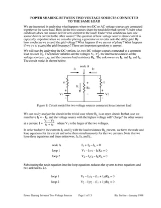
1. Power Sharing Between Two Voltage Sources Page 1 of 13 Ric Barline – January 1998
POWER SHARING BETWEEN TWO VOLTAGE SOURCES CONNECTED
TO THE SAME LOAD
We are interested in analyzing what happens when two DC or AC voltage sources are connected
together to the same load. How do the two sources share the total delivered current? Under what
conditions does one source deliver zero current to the load? Under what conditions does one
source deliver current to the other source? The question of how voltage sources share current is
especially important when we consider placing a generator or inverter onto the utility grid. By
how much can we exceed the grid voltage? What happens if we are out of phase? What happens
if we try to exceed the grid frequency? These are important questions to answer.
We will start by analyzing the DC version, i.e. two DC voltage sources connected to a common
load resistor RL. The known variables are the voltages V1,V2, the internal resistances of the
voltage sources r1, r2, and the common load resistance RL. The unknowns are I1, and I2, and IL.
The circuit model is shown below:
+
–
RL
r1 r2
+
–
+
–
V1 V2
I1 I2
IL
node A
Figure 1: Circuit model for two voltage sources connected to a common load
We can easily analyze the circuit in the trivial case where RL is an open circuit. In that case we
must have I1 = – I2, and the voltage source with the highest voltage will "charge" the other source
at a current I =
V1 – V2
r1 + r2
where V1 is the larger of the two voltages.
In order to derive the currents I1 and I2 with the load resistance RL present, we form the node and
loop equations for the circuit and solve them simultaneously for the two currents. Note that we
have three equations and three unknowns, I1, I2, and IL.
node A I1 + I2 – IL = 0
loop 1 V1 – I1r1 – ILRL = 0
loop 2 V2 – I2r2 – ILRL = 0
Substituting the node equation into the loop equations reduces the system to two equations and
two unknowns, i.e.
loop 1 V1 – I1r1 – (I1 + I2)RL = 0
loop 2 V2 – I2r2 – (I1 + I2)RL = 0

2. Power Sharing Between Two Voltage Sources Page 2 of 13 Ric Barline – January 1998
These equations may be solved for I1 and I2 to get:
I1 =
( )V1 – V2 RL + V1r2
( )r1 + r2 RL + r1r2
(1a)
I2 =
( )V2 – V1 RL + V2r1
( )r1 + r2 RL + r1r2
(2a)
IL = I1 + I2 =
V1r2 + V2r1
( )r1 + r2 RL + r1r2
(3a)
(Notice that in the limit of RL –> ∞ we obtain I1 = – I2 = I =
V1 – V2
r1 + r2
as we expect for the case
of RL is an open circuit.)
For simplicity at this point, we will let r1 = r2 = r, i.e. the internal resistances of the two sources
are equal. This would be the case for two identical generators. Then expressions (1a) through (3a)
simplify to:
I1 =
( )V1 – V2 RL + V1r
2rRL + r2 (1b)
I2 =
( )V2 – V1 RL + V2r
2rRL + r2 (2b)
IL =
V1 + V2
2RL + r (3b)
To make sense of these expressions, it is convenient to introduce the variables k1 and k2 which
represent the ratios V1:V2 and r:RL. These variables are defined as k1 =
V1
V2
and k2 =
r
RL
. Now
we can re-express expressions (1b) through (3b) in terms of k1 and k2:
I1 =
V2
RL
· f1(k1,k2) where f1(k1,k2) =
k1 – 1 + k1k2
2k2 + k2
2 (1)
I2 =
V2
RL
· f2(k1,k2) where f2(k1,k2) =
1 – k1 + k2
2k2 + k2
2 (2)
IL =
V2
RL
· f3(k1,k2) where f3(k1,k2) =
1 + k1
2 + k2
(3)
In these expressions, V2/RL was taken as the reference current, although V1/RL could just as
easily be used by dividing the functions by k1. The functions f1 through f3 are the coefficients of
the reference current as functions of the ratios k1 and k2 and contain all the information we need
to analyze the behavior of the circuit (but only for the special case of r1 = r2 = r).

3. Power Sharing Between Two Voltage Sources Page 3 of 13 Ric Barline – January 1998
In practical situations the internal resistance of the sources is much smaller than the load.
Therefore, we are primarily interested in the behavior of the functions f1, f2, and f3 at very small
values of k2 such as k2 = .05. Figure 2 below shows functions f1, f2, and f3 around k1 = 1 for the
value k2 = .05:
0.8 0.9 1 1.1 1.2
2
1
0
1
2
3
.488
0
f 1( ),k 1 k 2
f 2( ),k 1 k 2
f 3( ),k 1 k 2
1.051
k 1
Figure 2: Functions f1, f2, and f3 around k1 = 1 for k2 = .05
We are now in a position to answer the following questions:
• Under what conditions do the two sources share the load equally, i.e. when does I1 = I2? By
setting f1 = f2 and solving for k1 we obtain k1 = 1. Thus, I1 = I2 when V1 = V2. From figure 2
we see that at k1 = 1 we indeed have equal currents.
• When does I2 go to zero, and what is the value of I1 and IL at that point? By setting f2 = 0 and
solving for k1 we obtain k1 = 1 + k2. Thus, I2 will equal zero when V1/V2 = 1 + r/RL. From figure
2 we see that at k1 = 1 + .05 = 1.05 we indeed have f2 = 0. Substituting k1 = 1 + k2 into f1 gives f1
= 1, or I1 =
V2
RL
at that point. Since V2 is the voltage source that is not supplying any current, it
would be more interesting to express the current I1 in terms of its own source voltage V1 instead of
V2. To do this we multiply
V2
RL
by 1 =
1
k1
V1
V2
=
1
( )1 + k2
V1
V2
to get I1 =
V1
( )RL + r
. This is
exactly what we would expect in this case since the circuit reduces to the single source V1 driving
the load r + RL. Substituting k1 = 1 + k2 into f3 gives f3 = 1, or IL =
V2
RL
. Note that I1 = IL as
expected.
• When does I1 go to zero? By setting f1 = 0 and solving for k1 we obtain
1
k1
= 1 + k2. Thus, I1
will equal zero when V2/V1 = 1 + r/RL. From figure 2 we see that at k1 =
1
1 + .05 ≈ .95 we
indeed have f2 = 0. Substituting
1
k1
= 1 + k2 into f2 gives f2 =
1
( )1 + k2
, or I2 =
V2
RL
1
( )1 + k2
=
V2
( )RL + r
. Substituting
1
k1
= 1 + k2 into f3 gives the same result, so that I2 = IL as expected.

4. Power Sharing Between Two Voltage Sources Page 4 of 13 Ric Barline – January 1998
• Finally, what happens when k1 > 1 + k2? By substituting this inequality into f2, we obtain the
result that f2 < 0, i.e. I2 is negative. From figure 2 we see that at k1 > 1.05 we indeed have f2 < 0. At
that point f1 > 1, i.e. I1 >
V1
( )RL + r
. Similarly, when
1
k1
> 1 + k2, f1 < 0, i.e. I1 is negative, and I2
>
V1
( )RL + r
. This represents the two situations where one voltage source is not only delivering all
the current to the load but also delivering current to the other source.
Notice that the range of values of k1 that results in positive values for both I1 and I2 is
1
( )1 + k2
≤ k1 ≤ 1 + k2. This translates into a general rule: the smaller the ratio of r to RL, the
smaller the range of voltage ratios that will result in both sources delivering current. This rule
translates directly into the statement that low resistance sources must have closely matched
voltages in order to share current delivered to a load.
An example
When working through an example, we have to keep in mind that the voltages at the terminals of the
two sources are not V1 and V2, but rather V1 – I1r and V2 – I2r. In what follows we will refer to
these voltages as "terminal voltages" and V1 and V2 as "internal voltages". When two or more
sources are connected together in parallel, their terminal voltages must be equal since there is no
resistance separating them. It is also important to understand that the internal voltage and the
internal resistance do not actually exist apart from each other, i.e. we cannot get inside the voltage
sources and measure them seperately. We may treat them for analysis purposes as "lumped"
parameters, i.e. a perfect voltage source in series with a resistance, but in reality they are inextricably
mixed together. Also, the power delivered to the load, IL
2RL, is equal to the difference between the
total power being produced, V1I1 + V2I2, and the power delivered to the internal resistances, I1
2r +
I2
2r.
Assume two identical DC generators are on line together delivering power to a 10kW load at 100
volts and 100 amps. Each generator delivers 50A at 100V to the load. Assume each generator has
an internal resistance of .05 ohm . From ohm's law we know that the load has a resistance of 1
ohm, therefore we know that k2 = .05. Since each generator has an internal resistance of .05 ohm,
each generator drops 2.5V across its internal resistance, so each generator must have an internal
voltage of V1 = V2 = 102.5V.
Now assume we increase the throttle of generator A and increase its internal voltage until it takes
over all the load current, thereby completely unloading generator B. Under what conditions will this
occur? From our previous results we know that this will occur when k1 = 1 + k2, or when V1/V2 =
1.05. At I2 = 0, there will be zero volts dropped across the internal resistance of generator B, so its
internal voltage will be the same as its terminal voltage, i.e. V2 = ILRL = 100V. Therefore, generator
A will take over all the load current when its internal voltage is V1 = 1.05 x 100V = 105V.
Thus we see that as we increase the voltage of generator A, current is shifted away from generator
B, gradually unloading it, until at a 2.5V increase in the internal voltage of generator A, it takes over
the entire load and completely unloads generator B. Any further increase in the internal voltage of
generator A would reverse the current in generator B and operate it as a motor.
This effect of shifting the balance of power delivered by two sources is expected intuitively, but
we have discovered by this analysis the exact relationship between the internal generator voltage
ratio and the ratio between the internal and external resistances. For example, we now can say
immediately that if the internal resistances of the generators were .1 ohm, V1 of generator A
would have to go to exactly 110V in order to unload generator B.

5. Power Sharing Between Two Voltage Sources Page 5 of 13 Ric Barline – January 1998
Efficiency consideration
Consider the system efficiency for the two cases: a) both generators share the load equally, and
b) one generator takes all the load. In the first situation, the total power being produced is
2 x 102.5 x 50 = 10.25Kw, which divides into 10Kw to the load and 125 watts to each of the two
internal resistances. Notice that in the second situation, generator A is producing 105V x 100A =
10.5Kw, dividing into 10Kw to the load and 500 watts to its own internal resistance. This increase
in the power delivered to the internal resistances reduces the efficiency of the system, and illustrates
a general rule about power sharing: A system of power sources will have optimum efficiency when
they deliver current in proportion to the inverse of their internal resistances.
AC power sharing
An analysis of power sharing with AC sources is more complex than for DC sources, but builds
directly on the DC analysis. For simplicity we will not consider reactive loads here, only pure
resistive loads (the case of reactive loads will be left as an exercise). There are three questions that
we need to answer: what happens if we connect generator A and generator B, assuming equal
internal resistances, to a common load resistance under the following conditions: a) generators are
in–phase but have different voltages, b) generators have equal voltages but are out of phase, and c)
generators have equal voltages but have different frequencies?
To answer these questions we need to get a feel for the instantaneous differences V1(t) – V2(t)
between the voltage waveforms. The following plots show V1(t) – V2(t) for the three situations:
0 0.2 0.4 0.6 0.8 1
100
50
0
50
100
V 1( )t
V 2( )t
V 1( )t V 2( )t
t
Figure 5: Voltage difference between V1(t) = V1pksin(ωt) and V2(t) = V2pksin(ωt)

6. Power Sharing Between Two Voltage Sources Page 6 of 13 Ric Barline – January 1998
0 0.2 0.4 0.6 0.8 1
100
50
0
50
100
V 1( )t
V 2( )t
V 1( )t V 2( )t
t
Figure 6: Voltage difference between V1(t) = Vpksin(ωt) and V2(t) = Vpksin(ωt + φ)
0 0.2 0.4 0.6 0.8 1
100
50
0
50
100
V 1( )t
V 2( )t
V 1( )t V 2( )t
t
Figure 7: Voltage difference between V1(t) = Vpksin(ωt) and V2(t) = Vpksin[ ](ω+ϕ)t
Figure 5 shows two in–phase voltage waveforms with expressions V1(t) = V1pksin(ωt) and
V2(t) = V2pksin(ωt) with V1pk = 100V and V2pk = 95V, and ω = 2π rad/sec (1 rev/sec). Figure 6
shows two out–of–phase voltage waveforms with expressions V1(t) = Vpksin(ωt) and V2(t) =
Vpksin(ωt + φ) for Vpk = 100V and φ = .1rad. Figure 7 shows two off–frequency waveforms with
expressions V1(t) = Vpksin(ωt) and V2(t) = Vpksin[ ](ω+ϕ)t with ϕ = .1π rad/sec. The voltage
difference is a sinewave with magnitude Vpk and frequency ω + ϕ/2 that is modulated at a beat
frequency of ϕ/2.
Of much more interest than the voltage differences are the ratios k1(t) =
V1(t)
V2(t) . Knowledge of
these functions, and the constant value k2 = r/RL allows us to form expressions for the currents
I1(t), I2(t) and IL(t) for each of the three situations. Once we know these expressions we will be
able to answer our three questions precisely.

7. Power Sharing Between Two Voltage Sources Page 7 of 13 Ric Barline – January 1998
From the definitions of our various waveforms, we can form expressions for k1(t):
k11(t) =
V1(t)
V2(t) =
V1pksin(ωt)
V2pksin(ωt) for the in–phase generators with different peak voltages (5)
k12(t) =
V1(t)
V2(t) =
Vpksin(ωt)
Vpksin(ωt+φ) for the out–of–phase generators with equal peak voltages (6)
k13(t) =
V1(t)
V2(t) =
Vpksin(ωt)
Vpksin[ ](ω+ϕ)t
for the off–frequency generators (7)
These ratios are plotted below in figure 9 for the time range from t = 0 to t = 1 second (i.e. 360
electrical degrees):
0 0.2 0.4 0.6 0.8 1
0.5
1
1.5
k 11( )t
k 12( )t
k 13( )t
t
Figure 9: Voltage ratios k11(t), k12(t), and k13(t) as a function of time
This plot shows us what really happens to the voltage ratios over one cycle in our three situations:
a) for the in–phase generators with different peak voltages, the function k11(t) is a constant, i.e. the
voltage ratio is constant over time, at a value of approximately 1.05, as can be seen in figure 5. This
means that V2 is just a scaled–down version of V1 at all points in time.
b) for the out–of–phase generators the voltage ratio starts at zero (because V1 = 0 at t = 0) but
reaches 1 at t = .25 (ωt = π/2 or 90 electrical degrees), and then heads for +∞ as t –> .5 (because
V2 = 0 at t = .5), then snaps to –∞ at t = .5 (because suddenly V1 crosses over from positive to
negative), and then repeats itself exactly between t = .5 and t = 1, as can be seen in figure 6 also.
c) for the off–frequency generators the voltage ratio stays very close to 1 for most of the first half
cycle. Then, as t –> .5, the ratio heads for +∞ as V2 goes to zero. At t = .5 it snaps to –∞ and then
comes back to 1 at t = .75 (ωt = 3π/2 or 270 electrical degrees) and again heads for +∞ as t –> 1.
Note that unlike the function k12(t), the function k13(t) does not repeat itself from cycle to cycle, as
is clear from figure 7 also.
We are now in a good position to answer our three questions. Since we have expressions for k11(t),
k12(t), and k13(t), we can form time dependent expressions for the currents I1(t), I2(t), and IL(t) for
each of the three situations by combining expressions (5) through (7) with expressions (1) through
(3). These expressions will tell us exactly how our voltage sources are sharing power to the load.

8. Power Sharing Between Two Voltage Sources Page 8 of 13 Ric Barline – January 1998
For situation 1, we define the currents as I11(t), I12(t), and I1L(t), and obtain:
I11(t) =
sin(ωt)
RL
·
V1pk – V2pk + k2V1pk
k2(2 + k2) (8)
I12(t) =
sin(ωt)
RL
·
V2pk – V1pk + k2V2pk
k2(2 + k2) (9)
I1L(t) =
sin(ωt)
RL
·
V1pk + V2pk
2 + k2
(10)
For situation 2, we define the currents as I21(t), I22(t), and I2L(t), and obtain:
I21(t) =
Vpk
RL
·
sin(ωt) – sin(ωt + φ) + k2sin(ωt)
k2(2 + k2) (11)
I22(t) =
Vpk
RL
·
sin(ωt + φ) – sin(ωt) + k2sin(ωt + φ)
k2(2 + k2) (12)
I2L(t) =
Vpk
RL
·
sin(ωt) + sin(ωt + φ)
2 + k2
(13)
For situation 3, we define the currents as I31(t), I32(t), and I3L(t), and obtain:
I31(t) =
Vpk
RL
·
sin(ωt) – sin[ ](ω+ϕ)t + k2sin(ωt)
k2(2 + k2) (14)
I32(t) =
Vpk
RL
·
sin[ ](ω+ϕ)t – sin(ωt) + k2sin[ ](ω+ϕ)t
k2(2 + k2) (15)
I3L(t) =
Vpk
RL
·
sin(ωt) + sin[ ](ω+ϕ)t
2 + k2
(16)
We may plot these currents over one cycle for each of the three situations and see exactly how the
generators share current to the load in each situation. We will discover the interesting result that the
load current doesn't really care what the sources are doing, i.e. it remains the same in all three
situations even though the generator currents do not. Keep in mind that the sum of the generator
currents must always equal the load current. The following three plots assume k2 = .05.
(See next page)

9. Power Sharing Between Two Voltage Sources Page 9 of 13 Ric Barline – January 1998
0 0.2 0.4 0.6 0.8 1
100
50
0
50
100
I 11( )t
I 12( )t
I 1L( )t
t
Figure 10: Currents I1(t), I2(t), and IL(t) for V1(t) = V1pksin(ωt) and V2(t) = V2pksin(ωt)
0 0.2 0.4 0.6 0.8 1
100
50
0
50
100
I 21( )t
I 22( )t
I 2L( )t
t
Figure 11: Currents I1(t), I2(t), and IL(t) for V1(t) = Vpksin(ωt) and V2(t) = Vpksin(ωt + φ)

10. Power Sharing Between Two Voltage Sources Page 10 of 13 Ric Barline – January 1998
0 0.2 0.4 0.6 0.8 1
200
0
200
I 31( )t
I 32( )t
I 3L( )t
t
Figure 12: Currents I1(t), I2(t), and IL(t) for V1(t) = Vpksin(ωt) and V2(t) = Vpksin[ ](ω+ϕ)t
While interpreting these plots it is very helpful to look also at the corresponding voltage
waveforms in figures 5 through 7. Observe how the voltage differences translate into current
differences.
a) For the first case of in–phase generators with a voltage difference of 5 volts, the current
delivered by generator B is very near zero (actually it is 2.5A at its peak at t = .25) but sinusoidal,
and in a constant (negative) ratio with the current delivered by generator A. Although difficult to
make out in the plot, generator B is actually being charged by generator A at all times. Thus we
can conclude that generator B runs completely unloaded and in fact it actually runs as a motor, i.e.
delivers negative power all the time. The load current is sinusoidal at frequency ω, peak value of
approximately 95A, and is in phase with both voltage waveforms.
b) For the case of the equal voltage but out–of–phase generators, since generator B's voltage
waveform is alternately ahead of and then behind generator A's voltage waveforms, it starts out
slightly ahead of generator A and initially charges generator A at 110A . By time t = .25, both
voltages are equal, so their current are equal and positive. At this point they share the load. By
t = .5, the roles are reversed and generator A charges generator B. The result is that the generators
are alternately loaded and unloaded by each other. The peak generator currents are undoubtedly a
function of the phase angle, and would be larger with increased phase angle.
The load current is at frequency ω with a peak amplitude at t = .251 of approximately 97.5A.
Although it is difficult to see, the load current is phase shifted slightly with respect to both V1(t)
and V2(t), and in fact is exactly half-way between them (IL(t) has a phase angle of .05 radian,
which is exactly half of the phase angle of V2(t)). This makes sense because since both voltages
have the same amplitude, neither should affect the load phase angle any more than the other.
c) For the case of equal voltages but different frequencies, we can guess what will happen: Since
generator B is running slightly faster than generator A, its phase angle grows at the rate of ϕ. Its
voltage waveform is alternately ahead of and then behind generator A's voltage waveform (until it
catches back up after one "beat cycle"). Therefore, on the first rising quarter cycle, generator B
charges generator A. By about t = .25 the two generators share the load, and by about t = .4
generator A takes over the load completely. This situation is just like the previous one except that
the generators are phase shifted by an amount that increases with time. Therefore the peak value
of current is growing with time, as we guessed it would in the previous case. The amplitude will

11. Power Sharing Between Two Voltage Sources Page 11 of 13 Ric Barline – January 1998
continue to increase until time t = π/ϕ, and then decrease until at t = 2π/ϕ it returns to in-phase and
starts the process all over again. At its peak the current will reach extremely high values.
Notice, however, that while I1 and I2 are going crazy, IL is oblivious and remains perfectly
consistent with a peak of approximately 97.5A. Its phase angle is exactly half–way between the two
voltage waveforms, therefore its phase angle grows at a rate ϕ/2.
Reactive currents:
If we superimpose the voltage and current waveforms for the two generators, we find that only in
situation a) are the currents in phase with the voltages. This means that two generators that are out
of phase feeding the same load will be required to deliver reactive currents. The two figures below
show the phase relationship between voltage V1(t) and I1(t) for situations b) and c).
0 0.2 0.4 0.6 0.8 1
100
50
0
50
100
I 21( )t
V 1( )t
t
Figure 13: Phase relationship between V1(t) and I1(t) for situations b
0 0.2 0.4 0.6 0.8 1
200
100
0
100
200
I 31( )t
V 2( )t
t
Figure 13: Phase relationship between V1(t) and I1(t) for situations c)

12. Power Sharing Between Two Voltage Sources Page 12 of 13 Ric Barline – January 1998
What is evident from these plots is that in both cases there are large reactive currents flowing in
generator A. The corresponding currents flowing in generator B are not shown, but from figures
(10) through (12), we know that they are exactly the same except that their phase angle is opposite
that of generator A.
What we see in figure 12 is that while generator A is delivering current lagging the voltage,
generator B is receiving that current leading the voltage. This can be stated another way as
follows: generator A sees the load as inductive, while generator B sees the load as capacitive.
In situation c) the current initially lags, but because the phase is increasing with time, the phase
vector rotates (at angular velocity ϕ). Therefore, for 0 > t > π/ϕ the load looks inductive, then at
time t = π/ϕ it looks negative resistive, then for 2π/ϕ > t > 2π/ϕ the load looks capacitive. From
generator B's point of view, the situation is reversed.
Efficiency consideration:
Back on page 4 we stated a general proposition that a system of power sources will have optimum
efficiency when they deliver current in proportion to the inverse of their internal resistances. We
can now see why this is the case for AC power. Mismatches in phase or frequency cause currents
that are out of phase with the voltage that generates them, and this leads to VARS or volt-amps-
reactive. Currents that do not deliver power to the load still cause voltage drops and dissipation in
the internal resistances, so the ratio of power dissipated in the load to power dissipated in the
internal impedances increases as reactive power increases. Hence, efficiency is reduced. So an
efficiency rule may be stated in new terms for AC power: A system of AC power sources will
have optimum efficiency when they operate at the same voltage, phase angle and frequency.
Conclusions:
We have analyzed what happens when both DC and AC power sources are connected to the same
load. We have found that, in the DC case, one source "charges" the other according to certain
equations that involve the ratio of the voltages and the ratio of the source impedances to the load
impedance. In the AC case we determined that voltage imbalance causes no reactive currents, but
does cause one generator to become unloaded or even motored, a phase difference causes the load
to look reactive, and a frequency difference causes the load to look reactive with a phase angle that
changes with time at the frequency difference of the two waveforms.
We have one more thing to consider before we are finished with this subject, namely, throughout
this analysis we have been tacitly assuming that the generators are being driven by infinite
mechanical power sources, i.e. there is no inherent limit to the amount of current that can be
delivered to the load or to the other generator. This assumption of course is not valid, and we need
to understand what effect this has on the physical reality of connecting power sources in parallel.
We must also realize that we have greatly simplified this analysis over the real world by assuming
that both sources have equal internal resistances. Again this is invalid for the real world. The
internal resistance of a generator at Grand Coulee dam is quite a bit lower than that of a 1Kw
backup generator.
What would actually happen if we connected a 1Kw generator to the utility line, and tried to inject
out of phase or off frequency power? Obviously, Grand Coulee dam would win. It would be like
trying to push a locomotive with a golf cart. In terms of our analysis, here is what would happen:
Grand Coulee dam is generator A, our 1Kw generator is generator B, and the western United States
industrial complex is the load. Say we get our generator running at 3600 rpm (60Hz) and close a
transfer relay to the grid. If we are over voltage, the grid will look like an extremely low impedance,
i.e. we would be attempting to supply the entire load of the western US industrial complex (see
figure 10). If we are out of phase, we will operate into a highly inductive load (see figure 11). If we
are off frequency, we will operate into a load that quickly changed from inductive to capacitive (see
figure 12).

13. Power Sharing Between Two Voltage Sources Page 13 of 13 Ric Barline – January 1998
The best way to visualize this situation is to realize that Grand Coulee dam presents us with such a
"stiff" voltage source that the terminal voltage of our generator simply has no hope of being
anything else except what Grand Coulee says it is. Then the question we must ask is this: Can we
drive our generator hard enough to support an internal voltage that is arbitrarily different from the
terminal voltage? Well, the only way we can have a difference is to have a voltage drop across the
internal resistance of our generator. What would it take, for example, to have a terminal voltage of
95V and an internal voltage of 100V? If the internal resistance is .05 ohm, then it takes 100A to
support a 5 volt difference across it. But our little generator would have to produce 100A at 100
volts, or 10Kw in order to do this! Pretty hard for a 1Kw generator, although a 10Kw generator
could. So what would happen? Our generator would lug down until its speed and hence its internal
voltage reduced to whatever voltage difference it could support, i.e. it would lug down to an rpm at
which the power delivered to the load plus the power delivered to its own internal resistance did not
exceed 1Kw. This rpm would then determine the internal voltage of the generator.
Conversely, what if we connected to a 100V line with our rpm set to produce only 95V? In this case,
we would have to support -5V across the internal resistance, which would take –100A, or 100A into
our generator! So what would happen? The generator would act like a motor and speed up, thus
increasing its internal voltage to the point where it equaled the terminal voltage. The governor would
throttle back to zero as a result, and it would pull zero mechanical power. In fact we could shut the
gas engine off completely and it would still run!
These same things would happen if we went onto the grid either out of phase or off frequency.
Since the power sources feeding the grid are so big, just about anything we attach to them doesn't
have a chance of changing the grid voltage. So our device, whether it be a gas generator or an
inverter, would be forced to do whatever it takes internally to match the grid voltage waveform. In
the case of an inverter, it too has an ultimate driving source, for example a battery, and this source
has its own internal resistance. So the inverter may do its best to push on the grid but ultimately
will only be able to deliver as much current as it is designed for or the battery can supply. Once it
hits its limit, its voltage will be forced to conform to the grid.