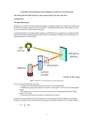
1. 3
Experiment 2: Determination of the Equilibrium Constant For Iron Thiocyanate
The data for this lab will be taken as a class to get one data set for the entire class.
I. Introduction
The Spectrophotometer
Substances are colored when they absorb a particular wavelength of light in the visible region and transmit
the other wavelengths. Complex ions such as FeSCN2+
usually absorb light in the visible range; the color
we see is the sum of the transmitted wavelengths.
A spectrophotometer is an instrument that separates visible light into its component wavelengths and then
measures the amount of light absorbed by the solution at a particular wavelength. The essential parts of a
spectrophotometer are shown below:
Figure 1: Schematic of the important parts of the spectrophotometer1
where the instrument has four main parts:
1. A light source that produces light with a range of visible wavelengths,
2. A diffraction grating and aperture that select one wavelength (λ = 447 nm) to pass through the
sample,
3. The sample that is stored in a cuvette with a precisely known and reproducible path length,
usually 1.00 cm and
4. A detector that measures the amount of light hitting its surface.
So what is it that the Spectronic 20 is measuring? It is measuring the amount of light that is transmitted
through your sample and hits the detector as a percentage of the light transmitted with a “blank” sample,
% T =
I
Io
×100%

2. 4
where %T is the percent transmittance, I is the amount of light that is transmitted through the sample and Io
is the amount of light transmitted through the blank, a sample that doesn’t absorb at all. What we would
like to know is slightly different: how much light is being absorbed by our sample? The absorbance is
defined as,
A = –log
I
Io
The absorbance, A, of an ideal solution is directly proportional to the concentration of absorbing ions or
molecules in that solution. The equation that relates absorbance to concentration is known as Beer’s Law,
A = ε l c (2)
where ε is called the extinction coefficient, an attribute that is specific to the absorbing species (at λ = 447
nm, ε is a constant), l is the width of the cuvette (another constant) which contains the solution that is being
analyzed and c is the concentration of the absorbing species expressed as molarity, M. The absorbing
species in this experiment is FeSCN2+
. Hence, the concentration, c, of FeSCN2+
is directly proportional to
the absorbance of that solution with a y-intercept equal to zero,
A = (constant) c (2)
The constant is the slope of the calibration curve made from the data in Procedure 1. Once the constant is
determined, you can measure the absorbance of any solution and then know its concentration of FeSCN2+
.
Let me restate this with direct reference to the procedure for this lab: once the calibration curve has been
constructed using Procedure 1, then any absorbance you measure in Procedure 3 can be used to calculate
the concentration of FeSCN2+
. It is the concentration of FeSCN2+
that is needed to then determine Kc for
reaction (1).
In this experiment, each group will use different cuvettes. It is imperative that the path length l is constant
for all of these cuvettes. Therefore, each of these cuvettes is made with a width that is precisely 1.00 cm.
Each cuvette is marked with a white line near the lip. This white line must be aligned precisely with the
black groove in the sample holder to ensure that the path length is 1.00 cm.
Determining The Equilibrium Constant
The main purpose of this lab is to determine the equilibrium constant for the complex ion formed by the
reaction of Fe3+
with SCN–
,
Fe3+
(aq) + SCN–
(aq) ↔ FeSCN2+
(aq) (1)
In this experiment, we will be calculating Kc for reaction (1) five different times. Each of those five times,
we will get a different number for Kc. While Kc for this reaction is constant, our attempts to experimentally
measure and calculate Kc will not be constant. There is experimental error, both procedural and human-
made, in this experiment. Therefore, we will take the average of the five experimentally determined values
of Kc.
As noted in lecture and the text, when Kc is >> 1, a reaction is product-favored, goes essentially to
completion and the concentrations of products at equilibrium are much larger than the concentration of
reactants (essentially, there are no reactants left). When Kc is <<1, a reaction is reactant-favored, does not
go at all and the concentrations of reactants at equilibrium are much larger than the concentration of
products (essentially, no products form).
As a hint to the answer for this lab, the value of Kc for reaction (1) is somewhere close to 1 (0.0001 < Kc <
10,000), meaning that the reaction gets stuck somewhere in the middle. What we will see is that we can

3. 5
manipulate the concentrations of reactants to make this reaction either go approximately 50% of the way to
completion or as far as 99.5% to completion. This is the basis for this experiment.
In Procedure 1, the above reaction will go essentially to completion. We will use LeChatelier’s Principle
(the subject of experiment 3-we’re just using it here) to drive the reaction to the right. We will add a known
concentration of Fe3+
. We will then add more than 100 times higher concentration of SCN–
than Fe3+
to the
reaction mixture. Using LeChatelier’s Principle, the excess SCN–
will push the position of equilibrium far
to the right and essentially to completion. The Fe3+
is the limiting reactant and all of the Fe3+
will be reacted
to produce FeSCN2+
. Therefore, the concentration of Fe3+
initially, after accounting for dilution, will be the
equilibrium or final concentration of FeSCN2+
.
As mentioned above when discussing the Spec 20, FeSCN2+
absorbs light at λ = 447 nm. We will construct
a “calibration” or “standard” curve that plots the known [FeSCN2+
] on the x-axis and the absorbance A of
FeCN2+
on the y-axis to establish a linear relationship between these two variables. The power of the
calibration curve is that for any solution containing FeSCN2+ as the only absorbing species, we can
measure the absorbance and use the linear relationship to calculate the [FeSCN2+
]. This is exactly why we
are preparing the calibration curve.
For Procedure 3, we add approximately equal concentrations of Fe3+
and SCN–
. Under these conditions, the
reaction will not go to completion. In fact, we will not know how far the reaction went to completion
because we don’t know the equilibrium constant Kc. However, if we measure the absorbance of the
unknown solutions in Procedure 3, then we can use the calibration curve prepared from Procedure 1 to
calculate what the equilibrium [FeSCN2+
] is in that solution. Once we have the equilibrium [FeSCN2+
], we
can fill in the rest of an ICE table to determine Kc.
To summarize, in this experiment we will:
1. Create a calibration curve by measuring the absorbance of a series of solutions of known
[FeSCN2+
]. For these solutions, reaction (1) will be essentially complete. The calibration should
yield a straight line relationship between [FeSCN2+
] and absorbance.
2. Measure the absorbance of a series of solutions for which [FeSCN2+
] is unknown. For these
solutions, reaction (1) will not be complete, but there is still the same relationship between
absorbance and concentration. Use this relationship and the absorbance to calculate [FeSCN2+
].
3. Determine the value of the equilibrium constant Kc for reaction (1).
II. Experimental
A. Equipment Needed:
From stock room: spectrophotometer cuvettes
Equipment in lab: Spectronic 20-D spectrophotometer, burets, aluminum foil
Chemicals in lab: 5.00×10–3
M KSCN in 0.500 M HCl, 2.00×10–3
M FeNO3 (or FeCl3) in 0.500
M HCl, 0.200 M KSCN in 0.500 M HCl and 0.500 M HCl
B. Disposal:
All chemicals used in this experiment should be disposed of in the proper waste container.
C. Experimental considerations
1. The product formed in this experiment is light sensitive. Direct sunlight will slowly decompose
the product, but room light will not. Use the aluminum foil to wrap around any flasks with
FeSCN2+
solution if you will be waiting for more than an hour to use the spectrophotometer
(which will most likely NOT happen).

4. 6
2. All of the ions in this experiment are dissolved in 0.500 M HCl to prevent the side reactions that
produce other complex ions. Henceforth, we will not mention this fact.
3. Please do not take any more of the standardized solutions than necessary.
D. Procedure 1. Preparing Standard Solutions for Absorbance Measurements.
The data for this procedure will be taken together as a class. For each volume of Fe(NO3)3, at
least three absorbance measurements will be taken. More may be taken if the first three
absorbance measurements are not approximately the same.
1. Turn on the spectrophotometer. It must warm up for 10–15 minutes.
2. Use the micropipette to deliver your assigned volume of 2.00×10–3
M Fe3+
into the 10 or 25 mL
graduated cylinder.
3. Add 2.0 mL of 0.200 M SCN–
to the graduated cylinder. Then dilute with 0.500 M HCl exactly
to the 10.00 mL mark. Use a dropper to deliver the last few drops of HCl
4. Use a glass stir rod to mix the solution until a uniform color is obtained. This may take 1-2
minutes of stirring
5. Pour ≈ 1 mL of solution into a cuvette. Rinse the walls of the cuvette with the solution by tilting
and rotating much like it was a 25 mL buret. Dispose of the 1 mL in a waste beaker. This is
necessary if the cuvette is not dry so that the solution you are putting into the cuvette is not diluted
by water left over in the cuvette from previous washings/measurements.
6. If the spectrophotometer has been warming up for 10-15 minutes, then begin testing the
solutions using procedure 2.
7. Repeat steps 2–5 for as many volumes as requested by the instructor until the instructor is
satisfied with the class’ data set.
E. Procedure 2: Measuring The Absorbance of the Standard Solutions.
1. To standardize the Spectronic 20 meter: 2-step standardizing procedure.
A. Set the wavelength dial to 447 nm. With the cell holder empty, adjust the left knob to
zero transmittance.
B. Fill a cuvette with 0.500 M HCl. Make sure you fill the cuvette more than halfway.
Wipe any fingerprints from the cuvette with a Kim-Wipe (and not a paper towel–the
paper towels scratch the cuvettes), and then place it in the cell holder. Ensure that the
vertical white mark on the cuvette is aligned with the mark in the spectrophotometer.
Close the cover for the sample holder. Adjust the lower right knob until the meter reads
100% transmittance. To scroll between %Transmittance and absorbance, press the
“Mode” button.
2. Rinse the cuvette with the solution to be measured, then fill the cuvette more than halfway.
3. Wipe off fingerprints from the cuvette with a Kim-Wipe. Place the cuvette into the sample
holder, replace the cap, and read and record in Table 1 (which should be taped in your notebook)
the ABSORBANCE, A, (% transmittance may also be recorded but, for our purposes, A has a
direct relationship to the quantity of interest, namely, concentration of iron thiocyanate).
4. Measure the absorbance A for each of the standard solutions.

5. 7
5. Calculate the diluted [Fe3+
] in each of the standard solutions using M1V1 = M2V2. Set this equal
to [FeSCN2+
] in the data table.
6. Once the instructor is satisfied that there will be no more measurements for this part of the lab,
determine the average and standard deviation for each mL of Fe3+
. Any values of absorbance that
are considerably different than the average should be tested using the Q test (see Appendix B:
Statistical Functions). If there are any values thrown out using the Q test, recalculate the average
and standard deviation without these points.
mL Fe3+
soln
(2.00 10–3
M)
diluted [Fe3+
]
=[FeSCN2+
]
Absorbance Values
at 447 nm
Average and
Standard deviation
of Absorbance
7. After approval of your data, discard the solutions into the container in the hood.
F. Procedure 3: Absorbance of Unknown Solutions
1. Prepare solutions with the volumes of 2.00×10–3
M Fe3+
and 5.00×10–3
M SCN–
(not the stuff
used in Procedure 1) indicated in Table A (below) in the graduated cylinder. Fill to 10.00 mL with
0.500 M HCl.
2. As determined by instructor, determine the absorbance of each solution and record the value in
Table 2 until a satisfactory data set is established.
Table A: Volumes for Unknown Solutions
Soln. mL of 2.00 10–3
M Fe3+
mL of 5.00 10–3
M SCN–
A 5 1
B 5 2
C 5 3
D 5 4
E 5 5

6. 8
Soln. mL of Fe3+
(2.00 10–3
M)
mL of SCN–
(5.00 10–3
M)
Absorbance
Values at 447
nm
Average and
Standard deviation
of Absorbance
A
B
C
D
E
III. Calculations
Approach to calculations for The Calibration Curve. For the standard solutions, the number of moles of
SCN–
is much greater than the number of moles of Fe3+
. Using LeChatelier’s Principle, the excess SCN–
drives reaction (1) to completion (or >99% of the way to completion). Therefore, for the standard solutions
used to prepare the calibration curve, Fe3+
is the limiting reactant and the initial concentration (accounting
for dilution to 10 mL) of Fe3+
is converted entirely to FeSCN2+
.
Approach to calculations for Determination of the Equilibrium Constant. For these solutions, the
number of moles of Fe3+
is approximately equal to the number of moles of SCN–
. In this case, we will
observe that the reaction does not go to completion. When a reaction does not go to completion, we can
count on setting up some kind of ICE table. The ICE tables and the equilibrium values of the concentrations
will allow us to determine the value for Kc, the equilibrium constant. Ideally, all of our calculations will
lead to similar values of Kc.
A. Calculating the concentration of a diluted solution.
This calculation will be used any time you mix solutions together to calculate the concentration of ions in
the new solution.
Ex: If 0.100 mL of 2.00×10–3
M SCN–
is diluted to a volume of 10.00 mL, what is the final
concentration of SCN–
ion?
M1V1 = M2V2
(2.00×10–3
M) (0.100 mL) = M2 (10.00 mL)
M2 = 2.00×10–5
M
Units on concentration and volume can be any units, as long as they cancel out.
B. Determining “conc. of FeSCN2+
final, (M)” for Table 4 from the calibration curve
In Table 2, there are five absorbance values. These absorbance values represent the absorbance of
FeSCN2+
. The calibration curve represents the relationship between conc. of FeSCN2+
and

7. 9
absorbance of FeSCN2+
. First, use Excel to find the equation of the line (y = mx + b) that relates
conc. (x) to absorbance (y). Then, use the absorbance values to plug into this equation and solve
for conc. Remember, it is impossible for the conc. of FeSCN2+
to be greater then the initial conc.
of either reacting species.
C. Calculating the value of the equilibrium constant from data in Table 2.
Suppose that [Fe3+
] = 8.0×10–4
M, [SCN–
] = 8.0×10–5
M, and that you determine from your
calibration curve that [FeSCN2+
] = 3.0×10–5
M. At this point, your MICE table looks like this:
M Fe3+
(aq) + SCN–
(aq) ↔ FeSCN2+
(aq)
I 8.0×10–4
8.0×10–5
0
C
E 3.0×10–5
From the three columns in Table 4, there is enough information to determine the value of Kc.
Because we know the initial concentration (we start with none) and the equilibrium concentration
of FeSCN2+
(we do assume that the reaction is at equilibrium by the time we get it into the
spectrophotometer, but this is a very good assumption born out by the fact that we don’t see the
color of the solutions changing with time), we can figure out the change in concentration of
FeSCN2+
. Since the change must be the same for all of them (taking into account coefficients), we
can fill in our table to make it look like this:
M Fe3+
(aq) + SCN–
(aq) ↔ FeSCN2+
(aq)
I 8.0 10–4
8.0 10–5
0
C –3.0×10–5
–3.0×10–5
+3.0×10–5
E 7.7×10–4
5.0×10–5
3.0 10–5
From here, we need to use the Kc expression for reaction (1) to get the value of Kc for this
reaction. Because reaction (1) forms complex ion FeSCN2+
, it is also called Kf (even though it
follows all the same rules as any Kc).
IV. Formatting Your Lab Notebook
A. Experiment title, date, your name and name of your partner. Page numbers for each page.
B. Introduction
1. What is the purpose of this lab?
2. Why does the reaction go to completion in Procedure 1 but not go to completion in Procedure 3
even though the value of Kc is constant in both procedures.
3. Handwritten procedure with spaces left open for each measurement and data table. Data tables
may be cut out and taped into the lab notebook or recreated by hand.
C. In Class Work
1. All data, averages and standard deviations must be calculated.
2. Hand-drawn plot of the calibration curve that takes up at least half a page in the notebook. If
your notebook does not have graph paper in it, then obtain a piece of graph paper from the
instructor, draw the graph on the paper and tape or staple the graph into your lab notebook.
D. Experimental Summary: in notebook before you leave lab
Were there any data points that had to be thrown out? Was your calibration curve linear?

8. 10
E. Results: at home
1. Calibration curve prepared by computer with best-fit line and R2
value displayed on graph.
Instructions on how to do this can be found in the introductory handout labeled “How to plot in
Excel.”
2. Calculations to determine [FeSCN2+
] in the unknown solutions.
3. ICE tables with Kc values for each of the 5 data points from Procedure 3.
4. Average and standard deviation values for Kc.
F. Experimental Summary: after all calculations are complete
Given that we don’t know the correct value of Kc for this experiment, and therefore can’t say
anything about accuracy, using standard deviation to assess precision how precise were your
values of Kc?
1
http://www.chem.vt.edu/chem-ed/spec/uv-vis/singlebeam.html accessed 8/12/05