SlideShare una empresa de Scribd logo
1 de 20
Descargar para leer sin conexión
18.1 Electric Charge
The electrical nature of matter is inherent in atomic
structure. An atom consists of a small, relatively massive
nucleus that contains particles called protons and
neutrons. A proton has a mass 1.673´ -
10 27
kg, while a
neutron has a slightly greater mass 1.675 10 kg.–27
´
Surrounding the nucleus is a diffuse cloud of orbiting
particles called electrons. An electron has a mass of
9.11 10 kg31
´ -
.
Like mass electric charge is an intrinsic property of
protons and electrons, and only two types of charge have
been discovered positive and negative. A proton has a
positive charge, and an electron has a negative charge. A
neutron has no net electric charge.
The magnitude of the charge on the proton exactly
equals the magnitude of the charge on the electron. The
proton carries a charge +e and the electron carries a
charge -e. The SI unit of charge is Coulomb( )C and e has
the value, e = ´ -
1.6 10 C19
Regarding charge following points are worth noting:
1. Like charges repel each other and unlike charges
attract each other.
2. Charge is a scalar and can be of two types positive
or negative.
3. Charge is quantized. The quantum of charge is e.
The charge on any body will be some integral
multiple of e, i.e.,
q ne= ±
where, n = ¼1 2 3, ,
Charge on any body can never be
1
3
e
æ
è
ç
ö
ø
÷ ,1.5e, etc.
Note
1. Apart from charge, energy, angular momentum and mass are also quantized.
The quantum of energy is hnand that of angular momentum is
h
2p
. Quantum
of mass is yet not known.
2. The protons and neutrons are combination of other entities called quarks,
which have charges 1
3
e and ±
2
3
e. However, isolated quarks have not been
observed, so, quantum of charge is still e.
4. During any process, the net electric charge of an
isolated system remains constant or we can say
that charge is conserved. Pair production and pair
annihilation are two examples of conservation of
charge.
5. A charge particle at rest produces electric field. A
charge particle in an unaccelerated motion
produces both electric and magnetic fields but
does not radiate energy. But an accelerated
charged particle not only produces an electric and
magnetic fields but also radiates energy in the
form of electromagnetic waves.
6. 1 Coulomb = ´ =3 109
esu
1
10
emu of charge.
18 Electrostatics
Chapter Snapshot
q Electric Charge
q Conductors and Insulators
q Charging of a Body
q Coulomb’s Law
q Electric Field
q Electric Potential Energy
q Electric Potential
q Relation between Electric Field and Potential
q Equipotential Surfaces
q Electric Dipole
q Gauss’s Law
q Properties of a Conductor
q Electric Field and Potential due to Charged Spherical Shell of Solid
Conducting Sphere
q Electric Field and Potential due to a Solid Sphere of Charge
q Capacitance
Get Discount Coupons for your Coaching institute and FREE Study Material at www.PICKMYCOACHING.com
Get Discount Coupons for your Coaching institute and FREE Study Material at www.PICKMYCOACHING.com1
www.pickM
yCoaching.com
Example 18.1 How many electrons are there in one coulomb
of negative charge?
Solution The negative charge is due to the presence of
excess electrons, since they carry negative charge. Because an
electron has a charge whose magnitude is e = ´ -
1.6 10 C19
, the
number of electrons is equal to the charge qdivided by the charge
e on each electron. Therefore, the number n of electrons is
n
q
e
= =
´ -
1.0
1.6 10 19
= ´6.25 1018
18.2 Conductors and Insulators
For the purpose of electrostatic theory all substances
can be divided into two main groups — conductors and
insulators. In conductors electric charges are free to move
from one place to another, whereas in insulators they are
tightly bound to their respective atoms. In an uncharged
body there are equal number of positive and negative
charges.
The examples of conductors of electricity are the
metals, human body and the earth and that of insulators
are glass, hard rubber and plastics. In metals, the free
charges are free electrons known as conduction electrons.
Semiconductors are a third class of materials, and
their electrical properties are somewhere between those of
insulators and conductors. Silicon and germanium are
well known examples of semiconductors.
18.3 Charging of a Body
Mainly there are following three methods of charging
a body:
(i) Charging by Rubbing
The simplest way to experience electric charges is to
rub certain bodies against each other. When a glass rod is
rubbed with a silk cloth the glass rod acquires some positive
charge and the silk cloth acquires negative charge by the
same amount. The explanation of appearance of electric
charge on rubbing is simple. All material bodies contain
large number of electrons and equal number of protons in
their normal state. When rubbed against each other, some
electrons from one body pass onto the other body. The body
that donates the electrons becomes positively charged
while that which receives the electrons becomes negatively
charged. For example when glass rod is rubbed with silk
cloth, glass rod becomes positively charged because it
donates the electrons while the silk cloth becomes
negatively charged because it receives electrons.
Electricity so obtained by rubbing two objects is also known
as frictional electricity. The other places where the
frictional electricity can be observed are when amber is
rubbed with wool or a comb is passed through a dry hair.
Clouds also become charged by friction.
(ii) Charging by Contact
When a negatively charged ebonite rod is rubbed on a
metal object, such as a sphere, some of the excess
electrons from the rod are transferred to the sphere. Once
the electrons are on the metal sphere, where they can
move readily, they repel one another and spread out over
the sphere’s surface. The insulated stand prevents them
from flowing to the earth. When the rod is removed the
sphere is left with a negative charge distributed over its
surface. In a similar manner the sphere will be left with a
positive charge after being rubbed with a positively
charged rod. In this case, electrons from the sphere would
be transferred to the rod. The process of giving one object a
net electric charge by placing it in contact with another
object that is already charged is known as charging by
contact.
(iii) Charging by Induction
It is also possible to charge a conductor in a way that
does not involve contact.
In Fig. (a) a negatively
charged rod brought close to (but
does not touch) a metal sphere. In
the sphere, the free electrons
close to the rod move to the other
side (by repulsion). As a result,
the part of the sphere nearer to
the rod becomes positively charged and the part farthest
from the rod negatively charged. This phenomenon is
called induction. Now if the rod is removed, the free
electrons return to their original places and the charged
regions disappear. Under most conditions the earth is a
2 Objective Physics Volume 2
––––––––
––––––––
– ––––– – –
–
–
– –– – –
–
–
–
–
–
––––
–
–
Ebonite rod
Metal
sphere
Insulated
stand
Fig. 18.1
––––––––
––––––––
Ebonite rod
Metal
sphere
Insulated
stand
(a) (b)
+
++
–––
+
+
+
+
+ ++
–
–
–
–
–– +
++
–––
+
+
+
+
+ ++
–
–
–
–
––
Grounding
wire
––––––––
––––––––
(c)
+
+
+ +
+
+
+
+
+ +
+
++
+
+
+
+
++
Earth
Fig. 18.2
– – – – – –
+ –
Plastic
Ebonite rod + –
+ –
+ –
+ –
Fig. 18.3
Get Discount Coupons for your Coaching institute and FREE Study Material at www.PICKMYCOACHING.com
Get Discount Coupons for your Coaching institute and FREE Study Material at www.PICKMYCOACHING.com2
www.pickM
yCoaching.com
good electric conductor. So when a metal wire is attached
between the sphere and the ground as in Fig. (b) some of
the free electrons leave the sphere and distribute
themselves on the much larger earth. If the grounding
wire is then removed, followed by the ebonite rod, the
sphere is left with a net positive charge. The process of
giving one object a net electric charge without touching
the object to a second charged object is called charging by
induction. The process could also be used to give the
sphere a net negative charge, if a positively charged rod
were used. Then, electrons would be drawn up from the
ground through the grounding wire and onto the sphere.
If the sphere were made from an insulating material
like plastic, instead of metal, the method of producing a
net charge by induction would not work, because very
little charge would flow through the insulating material
and down the grounding wire. However, the electric force
of the charged rod would have some effect as shown in
figure. The electric force would cause the positive and
negative charges in the molecules of the insulating
material to separate slightly, with the negative charges
being pushed away from the negative rod. The surface of
the plastic sphere does acquire a slight induced positive
charge, although no net charge is created.
Example 18.2 If we comb our hair on a dry day and bring
the comb near small pieces of paper, the comb attracts the
pieces, why?
Solution This is an example of frictional electricity and
induction. When we comb our hair it gets positively charged
by rubbing. When the comb is brought near the pieces of
paper some of the electrons accumulate at the edge of the
paper piece which is closer to the comb. At the farther end of
the piece there is deficiency of electrons and hence, positive
charge appears there. Such a redistribution of charge in a
material, due to presence of a nearby charged body is called
induction. The comb exerts larger attraction on the negative
charges of the paper piece as compared to the repulsion on
the positive charge. This is because the negative charges are
closer to the comb. Hence, there is a net attraction between
the comb and the paper piece.
Example 18.3 Does the attraction between the comb and the
piece of papers last for longer period of time?
Solution No, because the comb loses its net charge after
some time. The excess charge of the comb transfers to earth
through our body after some time.
Example 18.4 Can two similarly charged bodies attract
each other?
Solution Yes, when the charge on one body ( )q1 is much
greater than that on the other( )q2 and they are close enough to
each other so that force of attraction between q1 and induced
charge on the other exceeds the force of repulsion between q1
and q2 . However two similar point charges can never attract
each other because no induction will take place here.
Example 18.5 Does in charging the mass of a body change?
Solution Yes, as charging a body means addition or removal
of electrons and electron has a mass.
Example 18.6 Why a third hole in a socket provided for
grounding?
Solution All electric appliances may end with some charge
due to faulty connections. In such a situation charge will be
accumulated on the appliance. When the user touches the
appliance he may get a shock. By providing the third hole for
grounding all accumulated charge is discharged to the
ground and the appliance is safe.
18.4 Coulomb’s Law
The law that describes how charges interact with one
another was discovered by Charles Augustin de Coulomb
in 1785. With a sensitive torsion balance, Coulomb
measured the electric force between charged spheres. In
Coulomb’s experiment the charged spheres were much
smaller than the distance between them so that the
charges could be treated as point charges. The results of
the experiments of Coulomb and others are summarized in
Coulomb’s law.
The electric force Fe exerted by one point charge on
another acts along the line between the charges. It varies
inversely as the square of the distance separating the
charges and is proportional to the product of charges. The
force is repulsive if the charges have the same sign and
attractive if the charges have opposite signs.
The magnitude of the electric force exerted by a
charge q1 on another charge q2 a distance r away is thus,
given by
F
k q q
r
e =
| |1 2
2
…(i)
The value of the proportionality constant k in
Coulomb’s law depends on the system of units used. In SI
units the constant k is,
k 8.987551787 10
N-m
C
9
2
2
= ´
» ´8.988 10
N-m
C
9
2
2
The value of k is known to such a large number of
significant digits because this value is closely related to
the speed of light in vacuum. This speed is defined to be
exactly c 2.99792458 10 m / s8
= ´ . The numerical value of
k is defined in terms of c to be precisely.
k c=
æ
è
ç
ç
ö
ø
÷
÷
-
10 7
2
2
2N s
C
-
This constant k is often written as
1
4 0pe
, where e0
(epsilon-nought) is another constant. This appears to
complicate matters, but it actually simplifies many
formulae that we will encounter in later chapters. Thus,
Eq. (i) can be written as,
F
q q
r
e =
1
4 0
1 2
2
pe
| |
…(ii)
Chapter 18 · Electrostatics 3
Get Discount Coupons for your Coaching institute and FREE Study Material at www.PICKMYCOACHING.com
Get Discount Coupons for your Coaching institute and FREE Study Material at www.PICKMYCOACHING.com3
www.pickM
yCoaching.com
Here,
1
4 0pe
10
N - s
C
7
2
2
2
=
æ
è
ç
ç
ö
ø
÷
÷
-
c
Substituting value of c 2.99792458 10 m / s8
= ´ , we
get
1
4 0p e
= ´8.99 10 N - m /C9 2 2
In examples and problems we will often use the
approximate value,
1
4 0pe
9.0 10 N - m /C9 2 2
= ´
Here, the quantity e0 is called the permittivity of free
space. It has the value,
e0 = ´8.854 10 C /N - m–12 2 2
Regarding Coulomb’s law following points are worth
noting:
(1) Coulomb’s law stated above describes the
interaction of two point charges. When two
charges exert forces simultaneously on a third
charge, the total force acting on that charge is the
vector sum of the forces that the two charges would
exert individually. This important property, called
the principle of superposition of forces, holds for
any number of charges. Thus,
F F F Fnet
= + + ¼+1 2 n
(2) The electric force is an action reaction pair, i.e., the
two charges exert equal and opposite forces on
each other.
(3) The electric force is conservative in nature.
(4) Coulomb’s law as we have stated above can be
used for point charges in vacuum. If some
dielectric (insulator) is present in the space
between the charges, the net force acting on each
charge is altered
because charges
are induced in the
molecules of the
intervening
medium. We will
describe this effect later. Here at this moment it is
enough to say that the force decreases K times if
the medium extends till infinity. Here K is a
dimensionless constant which depends on the
medium and called dielectric constant of the
medium. Thus,
F
q q
r
e = ×
1
4 0
1 2
2
pe
(in vacuum)
F
F
K K
q q
r
e
e
¢ = = ×
1
4 0
1 2
2
pe
= ×
1
4
1 2
2
pe
q q
r
(in medium)
Here, e e= 0K is called permittivity of the medium.
Objective Galaxy 1 8 . 1
1. In few problems of electrostatics Lami’s theorem is very
useful.
According to this theorem, ‘if three concurrent forces F F1 2,
and F3 as shown in figure are in equilibrium or if
F F F1 2 2 0+ + = , then
F F F1 2 3
sin sin sina b g
= =
2. Suppose the position vectors of two charges q1 and q2 are r1
and r2
, then, electric force on charge q1 due to charge q2 is,
F
r r
r r1
0
1 2
1 2
3 1 1
1
4
= ×
pe
q q
| – |
( – )
Similarly, electric force on q2 due to charge q1 is
F
r r
r r2
0
1 2
2 1
3 2 1
1
4
= ×
pe
q q
| – |
( – )
Here q1 and q2 are to be substituted with sign.
r i j k1 1 1 1= + +x y z$ $ $
and r i j k2 2 2 2= + +x y z$ $ $
where ( , , )x y z1 1 1 and ( , , )x y z2 2 2 are the co-ordinates of
charges q1 and q2.
Example 18.7 What is the smallest electric force between
two charges placed at a distance of 1.0 m.
Solution F
q q
r
e = ×
1
4 0
1 2
2
pe
…(i)
For Fe to be minimum q q1 2 should be minimum. We know
that
( ) ( )min minq q1 2=
= e = ´ -
1.6 10 C19
Substituting in Eq. (i), we have
( )minFe =
´ ´ ´- -
(9.0 10 ) (1.6 10 ) (1.6 10 )
(1.
9 19 19
0)2
= ´ -
2.304 10 N28
Example 18.8 Three charges q C1 1= m , q C2 2= – m and
q C3 3= m are placed on the vertices of an equilateral triangle of
side 1.0 m. Find the net electric force acting on charge q1.
4 Objective Physics Volume 2
a
b
g
F1
F2
F3
Fig. 18.5
Fe q1
q2 Fe
In vacuum
r
Fig. 18.4
Get Discount Coupons for your Coaching institute and FREE Study Material at www.PICKMYCOACHING.com
Get Discount Coupons for your Coaching institute and FREE Study Material at www.PICKMYCOACHING.com4
www.pickM
yCoaching.com
How to Proceed Charge q2 will attract
charge q1 (along the line joining them)
and charge q3 will repel charge q1.
Therefore, two forces will act on q1, one
due to q2 and another due to q3 . Since,
the force is a vector quantity both of
these forces (say F1 andF2 ) will be added
by vector method. Following are two
methods of their addition.
Solution Method 1. In the figure,
| |F1 1
0
1 2
2
1
4
= = ×F
q q
rpe
= magnitude of force between andq q1 2
=
´ ´ ´- -
(9.0 10 ) (1.0 10 ) (2.0 10 )
(1.0)
9 6 6
2
= ´ -
1.8 10 N2
Similarly,
| |F2 2
0
1 3
2
1
4
= = ×F
q q
rpe
= magnitude of force between andq q1 2
=
´ ´ ´- -
(9.0 10 ) (1.0 10 ) (3.0 10 )
(1.0)
9 6 6
2
= ´ -
2.7 10 N2
Now, | | cosFnet = + + °F F F F1
2
2
2
1 22 120
= + +
æ
è
ç
ö
ø
÷
æ
è
ç
ç
ö
ø
÷
÷
(1.8) (2.7) 2 (1.8) (2.7) –
1
2
2 2
´ -
10 N2
= ´ -
2.38 10 N2
and tan
sin
cos
a =
°
+ °
F
F F
2
1 2
120
120
=
´
´ + ´ -
-
- -
(2.7 10 ) (0.87)
(1.8 10 ) (2.7 10 )
2
2 2 1
2
æ
è
ç
ö
ø
÷
or a = °79.2
Thus, the net force on charge q1 is 2.38 10 N2
´ -
at an
angle a = °79.2 with a line joining q1 and q2 as shown in
the figure.
Method 2. In this method let us assume a co-ordinate
axes with q1 at origin as shown in figure. The co-ordinates
of q q1 2, and q3 in this co-ordinate system are (0, 0, 0),
(1 m, 0, 0) and (0.5 m, 0.87 m, 0) respectively. Now,
F1 1 2= force on due to chargeq q
= ×
1
4 0
1 2
1 2
3 1 2
pe
q q
| – |
( – )
r r
r r
=
´ ´ ´(9.0 10 ) (1.0 10 ) (–2.0 10 )
(1.0)
9 –6 –6
3
´ + +[( – ) $ ( – ) $ ( – ) $ ]0 1 0 0 0 0i j k
= ´ -
(1.8 10 2 $)i N
and F2 = force on due to charge1 3q q
= ×
1
4 0
1 3
1 3
3 1 3
pe
q q
| – |
( – )
r r
r r
=
´ ´ ´(9.0 10 ) (1.0 10 ) (3.0 10 )
(1.0)
9 –6 –6
3
´ + +[( – $ ( – ) $ ( – ) $]0 0 0 00.5) 0.87i j k
= ´ -
( – $ – $)1.35 2.349i j 10 2
N
Therefore, net force on q1 is,
F F F= +1 2
= ´( $ $ –
0.45 – 2.349 ) 10i j 2
N
Note Once you write a vector in terms of $, $i j and $k, there is no need of writing the
magnitude and direction of vector separately.
Example 18.9 Two identical balls each having a density r
are suspended from a common point by two insulating strings
of equal length. Both the balls have equal mass and charge. In
equilibrium each string makes an angle q with vertical. Now,
both the balls are immersed in a liquid. As a result the angle q
does not change. The density of the liquid is s. Find the
dielectric constant of the liquid.
Solution Each ball is in equilibrium under the following
three forces:
(i) tension
(ii) electric force and
(iii) weight
So, Lami’s theorem can be applied.
Chapter 18 · Electrostatics 5
q1 q2
q3
Fig. 18.6
q1 q2
q3
a
120°
F1
F2 Fnet
Fig. 18.7
q1 q2
q3y
x
Fig. 18.8
In vacuum
Fe
q
q
w
T
In liquid
Fe¢
q
q
w ¢
T ¢
Fig. 18.9
Get Discount Coupons for your Coaching institute and FREE Study Material at www.PICKMYCOACHING.com
Get Discount Coupons for your Coaching institute and FREE Study Material at www.PICKMYCOACHING.com5
www.pickM
yCoaching.com
In the liquid, F
F
K
e
e
¢ =
where, K = dielectric constant of liquid
and w w¢ = - upthrust
Applying Lami’s theorem in vacuum
w Fe
sin ( ) sin ( )90 180° +
=
° -q q
or
w Fe
cos sinq q
= …(i)
Similarly in liquid,
w Fe¢
=
¢
cos sinq q
…(ii)
Dividing Eq. (i) by Eq. (ii), we get
w
w
F
F
e
e
¢
=
¢
or K
w
w
=
– upthrust
as
F
F
Ke
e¢
=
æ
è
ç
ç
ö
ø
÷
÷
=
V g
V g V g
r
r s–
(V = volume of ball)
or K =
-
r
r s
Note In the liquid Fe and w have been changed. Therefore, T will also change.
18.5 Electric Field
A charged particle cannot directly interact with
another particle kept at a distance. A charge produces
something called an electric field in the space around it
and this electric field exerts a force on any other charge
(except the source charge itself) placed in it.
Thus, the region surrounding a charge or distribution
of charge in which its electrical effects can be observed is
called the electric field of the charge or distribution of
charge. Electric field at a point can be defined in terms of
either a vector function E called electric field strength or a
scalar function V called electric potential. The electric
field can also be visualised graphically in terms of lines of
force.
Electric Field Strength ( )E
Like its gravitational counterpart, the electric field
strength (often called electric field) at a point in an electric
field is defined as the electrostatic forceFe per unit positive
charge. Thus, if the electrostatic force experienced by a
small test charge q0 isFe, then field strength at that point is
defined as,
E
F
=
®
lim
q
e
q0 0
0
The electric field is a vector quantity and its direction
is the same as the direction of the forceFe on a positive test
charge. The SI unit of electric field is N/C. Here, it should
be noted that the test charge q0 does not disturb other
charges which produces E. With the concept of electric
field, our description of electric interactions has two parts.
First, a given charge distribution acts as a source of
electric field. Second, the electric field exerts a force on
any charge that is present in this field.
An Electric Field Leads to a Force
Suppose there is an electric field strength E at some
point in an electric field, then the electrostatic force acting
on a charge +q is qE in the direction of E, while on the
charge – q it is qE in the opposite direction of E.
Example 18.10 An electric field of 105
N/C points due west
at a certain spot. What are the magnitude and direction of the
force that acts on a charge of + 2 mC and - 5 mC at this spot?
Solution Force on + =2 mC qE
= ´( )( )–
2 10 106 5
= 0.2N (due west)
Force on – C5 m = ´(5 10 ) (10 )–6 5
= 0.5 N (due east)
Electric Field Due to a Point Charge
The electric field produced by a point charge q can be
obtained in general terms from Coulomb’s law. First note
that the magnitude of the force exerted by the charge q on
a test charge q0 is,
F
qq
r
e = ×
1
4 0
0
2
p e
then divide this value by q0 to obtain the magnitude of
the field.
E
q
r
= ×
1
4 0
2
pe
If q is positive E is directed away from q. On the other
hand if q is negative, then E is directed towards q.
The electric field at a point is a vector quantity.
Suppose E1 is the field at a point due to a charge q1 and E2
is the field at the same point due to a charge q2. The
resultant field when both the charges are present is
E E E= +1 2
6 Objective Physics Volume 2
+
r q0
Fe
q
+ Eq
–q
E
Fig. 18.10
Get Discount Coupons for your Coaching institute and FREE Study Material at www.PICKMYCOACHING.com
Get Discount Coupons for your Coaching institute and FREE Study Material at www.PICKMYCOACHING.com6
www.pickM
yCoaching.com
If the given charge distribution is continuous, we can
use the technique of integration to find the resultant
electric field at a point.
Example 18.11 Two positive point charges q C1 16= m and
q C2 4= m , are separated in vacuum by a distance of 3.0 m.
Find the point on the line between the charges where the net
electric field is zero.
Solution Between the charges the two field contributions
have opposite directions, and the net electric field is zero at a
point (say P), where the magnitudes of E1 and E2 are equal.
However, since, q q2 1< , point P must be closer to q2 , in order
that the field of the smaller charge can balance the field of the
larger charge.
At P, E E1 2=
or
1
4
1
40
1
1
2
0
2
2
2
pe pe
q
r
q
r
= ×

r
r
q
q
1
2
1
2
=
= =
16
4
2 …(i)
Also, r r1 2+ = 3.0 m …(ii)
Solving these equations, we get
r1 2 m=
and r2 1 m=
Thus, the point P is at a distance of 2 m from q1 and 1 m
from q2 .
Electric Field of a Ring of Charge
Electric field at distance x from the centre of uniformly
charged ring of total charge q on its axis is given by,
E
qx
x R
x =
æ
è
çç
ö
ø
÷÷ +
1
4 0
2 2 3 2
pe ( ) /
Direction of this electric field is along the axis and
away from the ring in case of positively charged ring and
towards the ring in case of negatively charged ring.
From the above expression, we can see that
(i) Ex = 0 at x = 0, i.e., field is zero at the centre of the
ring. We should expect this, charges on opposite
sides of the ring would push in opposite directions
on a test charge at the centre, and the forces would
add to zero.
(ii) E
q
x
x = ×
1
4 0
2
pe
for x R>> , i.e., when the point P is
much farther from the ring, its field is the same as
that of a point charge. To an observer far from the
ring, the ring would appear like a point, and the
electric field reflects this.
(iii) Ex will be maximum where
dE
dx
x
= 0. Differentiating
Ex w.r.t. x and putting it equal to zero, we get
x
R
=
2
and Emax comes out to be,
2
3
1
43
0
2
pe
×
æ
è
çç
ö
ø
÷÷
q
R
.
Electric Field of an Infinitely Long Line
Charge
Electric field at distance r from an infinitely long line
charge is given by
E
r
=
l
pe2 0
Here l is charge per unit length. Direction of this
electric field is away from the line charge in case of
positively charged line charge and towards the line charge
in case of negatively charged line charge.
or E
r
µ
1
Thus, E-r graph is as shown in Fig. 18.15.
The direction of E is radially outward from the line.
Chapter 18 · Electrostatics 7
+
+
+
+
+
+
+ +
+
+
+
+
Ex P
Exx x
R R
Fig. 18.12
R
2
Ex
Emax
x
Fig. 18.13
+
+
+
+
+
+
+
+
+
+
+
+
+
+
+
+
+
+
E
l l
r
P
P
Er
Fig. 18.14
E
r
Fig. 18.15
+
PE2
q1 +
E1
q2
r1 r2
Fig. 18.11
Get Discount Coupons for your Coaching institute and FREE Study Material at www.PICKMYCOACHING.com
Get Discount Coupons for your Coaching institute and FREE Study Material at www.PICKMYCOACHING.com7
www.pickM
yCoaching.com
Example 18.12 A charge q C=1m is placed at point
( , , )1 2 4m m m. Find the electric field at point P m m m( , – , )0 4 3 .
Solution Here, rq = + +$ $ $i j k2 4
and rp = +– $ $4 3j k
 r rp q– – $ – $ – $= i j k6
or | – | (– ) (– ) (– )r rp q = + +1 6 12 2 2
= 38 m
Now, E = ×
1
4 0
3
pe
q
p q
p q
| – |
( – )
r r
r r
Substituting the values, we have
E i j k=
´ ´( )( )
( )
(–$ – $ – $)
–
/
9.0 1.010 10
38
6
9 6
3 2
= ( $ $ $)–38.42 – 230.52 – 38.42i j k
N
C
Electric Field Lines
As we have seen, electric charges create an electric
field in the space surrounding them. It is useful to have a
kind of map that gives the direction and indicates the
strength of the field at various places. Field lines, a
concept introduced by Michael Faraday, provide us with
an easy way to visualize the electric field.
“An electric field line is an imaginary line or curve
drawn through a region of space so that its tangent at any
point is in the direction of the electric field vector at that
point. The relative closeness of the lines at some place
give an idea about the intensity of electric field at that
point.”
The electric field lines have the following properties:
1. The tangent to a line at any point gives the
direction of E at that point. This is also the path on
which a positive test charge will tend to move if
free to do so.
2. Electric field lines always begin on a positive
charge and end on a negative charge and do not
start or stop in midspace.
3. The number of lines leaving a positive charge or
entering a negative charge is proportional to the
magnitude of the charge. This means, for example
that if 100 lines are drawn leaving a + 4 mC charge
then 75 lines would have to end on a –3 mCcharge.
4. Two lines can never intersect. If it happens then
two tangents can be drawn at their point of
intersection, i.e., intensity at that point will have
two directions which is absurd.
8 Objective Physics Volume 2
EQ
Ep
P
Q
A
| | | |E EA B>
B
Fig. 18.16
Objective Galaxy 1 8 . 2
1. Suppose a charge q is placed at a point whose position vector is rq and we want to find the electric field at a point P whose position
vector is rp Then in vector form the electric field is given by,
E
r r
r r= ×
1
4 0
3
pe
q
p q
p q
| – |
( – )
Here, r i j zp p p px y z= + +$ $ $
and r i j kq q q qx y z= + +$ $ $
q –q
(a) (b)
(c)
+ –
q q
+
(d)
+qq
–
(e)
–q –q + q2q –
(f)
Fig. 18.17
Get Discount Coupons for your Coaching institute and FREE Study Material at www.PICKMYCOACHING.com
Get Discount Coupons for your Coaching institute and FREE Study Material at www.PICKMYCOACHING.com8
www.pickM
yCoaching.com
5. In a uniform field, the field lines are straight
parallel and uniformly spaced.
6. The electric field lines can never form closed loops
as a line can never start and end on the same
charge.
7. Electric field lines also give us an indication of the
equipotential surface (surface which has the same
potential)
8. Electric field lines always flow from higher
potential to lower potential.
9. In a region where there is no electric field, lines are
absent. This is why inside a conductor (where
electric field is zero) there, cannot be any electric
field line.
10. Electric lines of force ends or starts normally from
the surface of a conductor.
18.6 Electric Potential Energy
If the force F is conservative, the work done by F can
always be expressed in terms of a potential energy U.
When the particle moves from a point where the potential
energy is Ua to a point where it is Ub, the change in
potential energy is, DU U Ub a= – . This is related by the
work Wa b® as
W U U U U Ua b a b b a® = = =– – ( – ) – D …(i)
Here Wa b® is the work done in displacing the particle
from a to b by the conservative force (here electrostatic)
not by us. Moreover we can see from Eq. (i) that if Wa b® is
positive, DU is negative and the potential energy
decreases. So, whenever the work done by a conservative
force is positive, the potential energy of the system
decreases and vice versa. That’s what happens when a
particle is thrown upwards, the work done by gravity is
negative, and the potential energy increases.
Example 18.13 A uniform electric field E0 is directed along
positive y-direction. Find the change in electric potential
energy of a positive test charge q0 when it is displaced in this
field from y ai = to y af = 2 along the y-axis.
Solution Electrostatic force on the test charge,
F q Ee = 0 0 (along positive y-direction)
 W Ui f- = – D
or DU Wi f= -– = – [ ( – )]q E a a0 0 2
= – q E a0 0
Note Here work done by electrostatic force is positive. Hence, the potential
energy is decreasing.
Electric Potential Energy of Two Charges
The idea of electric potential energy is not restricted to
the special case of a uniform electric field as in example
18.13. Let us now calculate the work done on a test charge
q0 moving in a non-uniform electric field caused by a
single, stationary point charge q.
The Coulomb’s force on q0 at a distance r from a fixed
charge q is,
F
qq
r
= ×
1
4 0
0
2
pe
If the two charges have same signs, the force is
repulsive and if the two charges have opposite signs, the
force is attractive. The force is not constant during the
displacement, so we have to integrate to calculate the
work Wa b® done on q0 by this force as q0 moves from a to b.
 W F dra b r
r
a
b
® = ò = ×ò
1
4 0
0
2
per
r
a
b qq
r
dr
=
æ
è
çç
ö
ø
÷÷
qq
r ra b
0
04
1 1
pe
–
Being a conservative force this work is path
independent. From the definition of potential energy,
U U Wb a a b– –= -
=
æ
è
çç
ö
ø
÷÷
qq
r rb a
0
04
1 1
pe
–
We choose the potential energy of the two charge
system to be zero when they have infinite separation. This
meansU¥ = 0. The potential energy when the separation is
r is Ur
 U U
qq
r
r – –¥ =
¥
æ
è
ç
ö
ø
÷0
04
1 1
pe
or U
qq
r
r = 0
04
1
pe
This is the expression for electric potential energy of
two point charges kept at a separation r. In this expression
both the charges q and q0 are to be substituted with sign.
Electric Potential Energy of a System of
Charges
To find electrical potential energy of a system of
charges, we make pairs. If there are total n charges then
total number of pairs are
n n( )
.
-1
2
Neither of the pair should
be repeted, nor should be left.
Chapter 18 · Electrostatics 9
E0
q E0 0
+ q0
Fig. 18.18
q
a
q0
b
r
ra
rb
Fig. 18.19
Get Discount Coupons for your Coaching institute and FREE Study Material at www.PICKMYCOACHING.com
Get Discount Coupons for your Coaching institute and FREE Study Material at www.PICKMYCOACHING.com9
www.pickM
yCoaching.com
For example electric potential energy of four point
charges q q q1 2 3, , and q4 would be given by,
U
q q
r
q q
r
q q
r
q q
r
q q
r
q q
= + + + + +
1
4 0
4 3
43
4 2
42
4 1
41
3 2
32
3 1
31
2
pe
1
21r
é
ë
ê
ù
û
ú
…(ii)
Here, all the charges are to be substituted with sign.
Example 18.14 Four charges q C1 1= m , q C2 2= m ,
q C3 3= – m and q C4 4= m are kept on the vertices of a square of
side 1 m. Find the electric potential energy of this system of
charges.
Solution In this problem,
r r r r41 43 32 21 1= = = = m
and r r42 31
2 2
1 1 2= = + =( ) ( ) m
Substituting the proper values with sign in Eq. (ii), we get
U = ´( )( )( )– –
9.0 10 10 109 6 6
(4)(–3)
1
(4)(2)
2
(4)(1)
1
(–3)(2)
1
(–3)(1)
2
+ + + +
(2)(1)
1
+
é
ëê
ù
ûú
= ´ +
é
ëê
ù
ûú(9.0 10 12
5
2
3–
) – = ´– 7.62 10 J–2
Note Here negative sign of U implies that positive work has been done by
electrostaticforcesinassemblingthesechargesatrespectivedistancesfrominfinity.
Example 18.15 Two point charges are located on the x-axis,
q C1 1= – m at x = 0 and q C2 1= + m at x m=1 .
(a) Find the work that must be done by an external force to
bring a third point charge q C3 1= + m from infinity to
x m= 2 .
(b) Find the total potential energy of the system of three
charges.
Solution (a) The work that must be done on q3 by an
external force is equal to the difference of potential energy U
when the charge is at x = 2 m and the potential energy when it
is at infinity.
 W U Uf i= – = + +
é
ë
ê
ù
û
ú
1
4 0
3 2
32
3 1
31
2 1
21pe
q q
r
q q
r
q q
rf f f( ) ( ) ( )
–
( ) ( ) ( )
1
4 0
3 2
32
3 1
31
2 1
21pe
q q
r
q q
r
q q
ri i i
+ +
é
ë
ê
ù
û
ú
Here, ( ) ( )r ri f21 21= and ( ) ( )r ri i32 31= = ¥
 W
q q
r
q q
rf f
= +
é
ë
ê
ù
û
ú
1
4 0
3 2
32
3 1
31pe ( ) ( )
Substituting the values, we have
W = ´ +(9.0 10 ) (10 )
(1) (1)
(1.0)
(1) (–1)
(2.0
9 –12
)
é
ë
ê
ù
û
ú
= ´4.5 10 J–3
(b) The total potential energy of the three charges is
given by,
U
q q
r
q q
r
q q
r
= + +
æ
è
çç
ö
ø
÷÷
1
4 0
3 2
32
3 1
31
2 1
21pe
= ´ + +(9.0 10 )
(1) (1)
(1.0)
(1) (–1)
(2.0)
(1) (9 –1)
(1.0)
(1
é
ë
ê
ù
û
ú 0 12–
)
= ´– 4.5 10–3
J
Example 18.16 Two point charges q q C1 2 2= = m are fixed
at x m1 3= + and x m2 3= – as shown in figure. A third particle
of mass 1 g and charge q C3 4= – m are released from rest at
y m= 4.0 . Find the speed of the particle as it reaches the
origin.
How to Proceed Here the charge q3 is attracted towards q1
and q2 both. So, the net force on q3 is towards origin.
By this force charge is accelerated towards origin, but this
acceleration is not constant. So, to obtain the speed of particle
at origin by kinematics, we will have to find first the
acceleration at same intermediate position and then will have
to integrate it with proper limits. On the other hand it is easy
to use energy conservation principle as the only forces are
conservative.
10 Objective Physics Volume 2
1 m
1 m
q1 q2
q3q4
Fig. 18.20 y
x
q2 q1
x1 = 3 mx2 = –3 m
O
q3 y = 4 m
Fig. 18.21
y
x
q2 q1
O
q3
Fnet
Fig. 18.22
q2
q3
q1
q4
Get Discount Coupons for your Coaching institute and FREE Study Material at www.PICKMYCOACHING.com
Get Discount Coupons for your Coaching institute and FREE Study Material at www.PICKMYCOACHING.com10
www.pickM
yCoaching.com
Solution Let v be the speed of particle at origin. From
conservation of mechanical energy,
U K U Ki i f f+ = +
or
1
4
0
0
3 2
32
3 1
31
2 1
21pe
q q
r
q q
r
q q
ri i i( ) ( ) ( )
+ +
é
ë
ê
ù
û
ú +
= + +
é
ë
ê
ù
û
ú +
1
4
1
20
3 2
32
3 1
31
2 1
21
2
pe
q q
r
q q
r
q q
r
mv
f f f( ) ( ) ( )
Here, ( ) ( )r ri f21 21=
Substituting the proper values, we have
(9.0 10 )
(– 4) (2)
(5.0)
(– 4) (2)
(5.0)
9
´ +
é
ë
ê
ù
û
ú ´ 10–12
= ´ +
é
ë
ê
ù
û
ú(9.0 10 )
(– 4) (2)
(3.0)
(– 4) (2)
(3.0)
9
10
1
2
10–12 –3
´ + ´ ´ v2
 ( ) – ( ) –– – –
9 10
16
5
9 10
16
3
1
2
103 3 3 2
´
æ
è
ç
ö
ø
÷ = ´
æ
è
ç
ö
ø
÷ + ´ ´ v
( )( )– –
9 10 16
2
15
1
2
103 3 2
´
æ
è
ç
ö
ø
÷ = ´ ´ v
 v = 6.2 m s/
18.7 Electric Potential
As we have discussed in Article 18.5 that an electric
field at any point can be defined in two different ways:
(i) by the field strength E, and
(ii) by the electric potential V at the point under
consideration.
Both E and V are functions of position and there is a
fixed relationship between these two. Of these, the field
strengthEis a vector quantity while the electric potential V
is a scalar quantity. In this article we will discuss about the
electric potential and in the next the relationship between
E and V. Potential is the potential energy per unit charge.
Electric potential at any point in an electric field is defined
as the potential energy per unit charge, same as the field
strength is defined as the force per unit charge. Thus,
V
U
q
=
0
or U q V= 0
The SI unit of potential is volt ( V ) which is equal to
joule per coulomb. So,
1 V 1 volt 1 J /C 1 joule / coulomb= = =
The work done by the electrostatic force in displacing
a test charge q0 from a to b in an electric field is defined as
the negative of change in potential energy between them,
or
DU Wa b= – –
 U U Wb a a b– – –=
We divide this equation by q0,
U
q
U
q
W
q
b a a b
0 0 0
- = –
–
or V V
W
q
a b
a b
–
–
=
0
as V
U
q
=
0
Thus, the work done per unit charge by the electric
force when a charged body moves from a to b is equal to
the potential at a minus the potential at b. We sometimes
abbreviate this difference as V V Vab a b= – .
Another way to interpret the potential difference Vab is
that the potential at a minus potential at b, equals the work
that must be done to move a unit positive charge slowly
from b to a against the electric force.
V V
W
q
a b
b a
–
( )–
=
external force
0
Absolute Potential at Some Points
Suppose we take the point b at infinity and as a
reference point assign the value Vb = 0, the above
equations can be written as
V V
W
q
W
q
a b
a b b a
–
( ) ( )– –
= =
electric force external force
0 0
or V
W
q
W
q
a
a a
= =
¥ ¥( ) ( )– –electric force external force
0 0
Thus, the absolute electric potential at point a in an
electric field can be defined as the work done in displacing
a unit positive charge from infinity to a by the external
force or the work done per unit positive charge in
displacing it from a to infinity.
Objective Galaxy 1 8 . 3
Following three formulae are very useful in the problems
related to work done in electric field.
( ) ( – )–W q V Va b a belectric force = 0
( ) ( – ) – ( )– –W q V V Wa b b a a bexternal force electric force= =0
( )–W q Va a¥ =external force 0
Here, q Va0, andVb are to be substituted with sign.
Example 18.17 The electric potential at point A is 20 V
and at B is – 40 V. Find the work done by an external force
and electrostatic force in moving an electron slowly from B
to A.
Solution Here, the test charge is an electron, i.e.,
q0 – 1.6 10 C–19
= ´
VA = 20 V
and VB = – 40 V
Work done by external force
( ) ( – )–W q V VB A A Bexternal force = 0
Chapter 18 · Electrostatics 11
Get Discount Coupons for your Coaching institute and FREE Study Material at www.PICKMYCOACHING.com
Get Discount Coupons for your Coaching institute and FREE Study Material at www.PICKMYCOACHING.com11
www.pickM
yCoaching.com
= ´(– 1.6 10 ) [(20) – (– 40)]–19
= ´– 9.6 10 J–18
Work done by electric force
( ) – ( )– –W WB A B Aelectric force external force=
= ´– (– 9.6 10 J)–18
= ´9.6 10 J–18
Note Here we can see that the electron (a negative charge) moves from B
(lower potential) to A (higher potential) and the work done by electric force is
positive. Therefore, we may conclude that whenever a negative charge moves
from a lower potential to higher potential work done by the electric force is
positive or when a positive charge moves from lower potential to higher
potential the work done by the electric force is negative.
Example 18.18 Find the work done by some external force
in moving a charge q C= 2 m from infinity to a point where
electric potential is104
V.
Solution Using the relation,
( )–W qVa a¥ =external force
We have, ( ) ( )( )–
–
W a¥ = ´external force 2 10 106 4
= ´2 10 2–
J
Electric Potential Due to a Point Charge q
From the definition of potential,
V
U
q
=
0
=
×
1
4 0
0
0
pe
q q
r
q
or V
q
r
= ×
1
4 0pe
Here, r is the distance from the point charge q to the
point at which the potential is evaluated.
If q is positive, the potential that it produces is positive
at all points; if q is negative, it produces a potential that is
negative everywhere. In either case, V is equal to zero at
r = ¥.
Electric Potential Due to a System of
Charges
Just as the electric field due to a collection of point
charges is the vector sum of the fields produced by each
charge, the electric potential due to a collection of point
charges is the scalar sum of the potentials due to each
charge.
V
q
r
i
ii
= å
1
4 0pe
Objective Galaxy 1 8 . 4
In the equationV
q
r
i
ii
= å
1
4 0pe
if the whole charge is at equal
distance r0 from the point where V is to be evaluated, then
we can write,
V
q
r
= ×
1
4 0 0pe
net
where qnet is the algebraic sum of all the charges of which
the system is made.
Here are few examples:
Examples 1. Four charges are placed on the vertices of a
square as shown in figure. The electric potential at centre of
the square is zero as all the charges are at same distance
from the centre and
qnet C C C C= +
=
4 2 2 4
0
m m m m– –
.
Example 2. A charge q is uniformly distributed over the
circumference of a ring in Fig. (a) and is non-uniformly
distributed in Fig. (b).
The electric potential at the centre of the ring in both the
cases is
V
q
R
= ×
1
4 0pe
(where R = radius of ring)
12 Objective Physics Volume 2
–2 Cm
+2 Cm–4 Cm
+4 Cm
Fig. 18.23
+
+
+
+
+
+
+
+
+
+
+
+
+
+
+
+
+
R
q
(a) (b)
++
+
+
+
+
+
+
+
+
+
+
R
q
+ +
+
+
+
+
Fig. 18.24
r
C P
R r2 2
+
R
Fig. 18.25
Get Discount Coupons for your Coaching institute and FREE Study Material at www.PICKMYCOACHING.com
Get Discount Coupons for your Coaching institute and FREE Study Material at www.PICKMYCOACHING.com12
www.pickM
yCoaching.com
and at a distance r from the centre of ring on its axis would
be,
V
q
R r
= ×
+
1
4 0
2 2pe
Example 18.19 Three point charges q C1 1= m , q C2 2= – m
and q C3 3= m are placed at (1 m, 0, 0), ( , , )0 2 0m and (0, 0, 3 m)
respectively. Find the electric potential at origin.
Solution The net electric potential at origin is,
V
q
r
q
r
q
r
= + +
é
ë
ê
ù
û
ú
1
4 0
1
1
2
2
3
3pe
Substituting the values, we have
V = ´ +
æ
è
ç
ö
ø
÷ ´(9.0 10 )
1
1.0
–
2
2.0
3
3.0
9
10 6–
= ´9.0 10 V3
Example 18.20 A charge q C=10 m is distributed uniformly
over the circumference of a ring of radius 3 m placed on x-y
plane with its centre at origin. Find the electric potential at a
point P(0, 0, 4 m).
Solution The electric potential at point P would be,
V
q
r
= ×
1
4 0 0pe
Here r0 = distance of point P from the circumference of
ring
= +( ) ( )3 42 2
= 5 m
and q =10 mC =10 5–
C
Substituting the values, we have
V =
´
= ´
(9.0 10 ) (10 )
(5.0)
1.8
9 –5
104
V
Variation of Electric Potential on the Axis
of a Charged Ring
We have discussed in
Medical Galaxy that the electric
potential at the centre of a
charged ring (whether charged
uniformly or non-uniformly) is
1
4 0pe
×
q
R
and at a distance r from
the centre on the axis of the ring
is
1
4 0
2 2pe
×
+
q
R r
.From these expressions we can see that
electric potential is maximum at the centre and decreases
as we move away from the centre on the axis. Thus
potential varies with distance r as shown in figure.
In the figure, V
q
R
0
0
1
4
= ×
pe
Example 18.21 Find out the points on the line joining two
charges + q and – 3q (kept at a distance of 1.0 m), where
electric potential is zero.
Solution Let P be the point on the axis either to the left or to
the right of charge + q at a distance r where potential is zero.
Hence,
V
q
r
q
r
P =
+
=
4
3
4 1
0
0 0pe pe
–
( )
Solving this, we get r = 0.5m
Further, V
q
r
q
r
P = =
4
3
4 1
0
0 0pe pe
–
( – )
,
which gives r = 0.25 m.
Thus, the potential will be zero at point P on the axis
which is either 0.5 m to the left or 0.25 m to the right of
charge + q.
18.8 Relation between Electric
Field and Potential
Let us first consider the case when electric potential V
is known and we want to calculate E. The relation is as
under,
In Case of Cartesian Coordinates
E i j k= + +E E Ex y z
$ $ $
Here, E
V
x
V xx =


=– – (partial derivative of wrt )
E
V
y
V yy =


=– – (partial derivative of wrt )
E
V
z
V zz =


=– – (partial derivative of wrt )
 E i j k= -


+


+


é
ë
ê
ù
û
ú
V
x
V
y
V
z
$ $ $
This is also sometimes written as,
E = – gradient V
= – grad V
Chapter 18 · Electrostatics 13
y
4 m
P
r0
3 m
q
x
z
+
+
+
++++
+
+
+
+
+
+ + +
+
Fig. 18.26
V0
V
rr = 0
Fig. 18.27
1.0 m –3qP +q
r
or
–3qP+q
r 1.0 – r
Fig. 18.28
Get Discount Coupons for your Coaching institute and FREE Study Material at www.PICKMYCOACHING.com
Get Discount Coupons for your Coaching institute and FREE Study Material at www.PICKMYCOACHING.com13
www.pickM
yCoaching.com
= Ñ– V
Example 18.22 The electric potential in a region is
represented as,
V x y z= +2 3 –
obtain expression for electric field strength.
Solution E i j k=


+


+


é
ë
ê
ù
û
ú– $ $ $V
x
V
y
V
z
Here,


=


+ =
V
x x
x y z( – )2 3 2


=


+ =
V
y y
x y z( – )2 3 3


=


+ =
V
z z
x y z( – ) –2 3 1
 E i j k= - -2 3 +$ $ $
We have determined how to calculate electric fieldE from
the electrostatic potential V. Let us now consider how to
calculate potential difference or absolute potential if
electric field E is known. For this use the relation,
dV d= ×– E r
or dV d
A
B
A
B
ò ò= ×– E r
or V V dB A A
B
– –= ×ò E r
Here, d dx dy dzr i j k$ $ $+ +
When E is Uniform
Let us take this case with the help of an example.
Example 18.23 Find Vab in an electric field
E i j k= + +( $ $ $)2 3 4
N
C
where r i j ka m= +($ – $ $)2
and r i j kb m= +( $ $ – $)2 2 .
Solution Here the given field is uniform (constant). So
using,
dV d= ×– E r
or V V V dab a b b
a
= = ×ò– – E r
= - + + × + +ò ( $ $ $) ( $ $ $)
( , ,– )
( ,– , )
2 3 4
2 1 2
1 2 1
i j k i j kdx dy dz
= + +ò– ( )
( , ,– )
( ,– , )
2 3 4
2 1 2
1 2 1
dx dy dz
= - + +[ ]( , , – )
( , – , )
2 3 4 2 1 2
1 2 1
x y z = – 1 volt
Note In uniform electric field we can also apply,
V Ed=
Here V is the potential difference between any two
points, E the magnitude of electric field and d is the
projection of the distance between two points along the
electric field.
For example, in the figure if we are interested in the
potential difference between points A and B we will have
to keep two points in mind,
(i) V VA B> as electric lines always flow from higher
potential to lower potential.
(ii) d AB¹ but d AC=
Hence, in the above figure, V V EdA B– = .
Example 18.24 In uniform electric field E =10 N C/ as
shown in figure, find :
(a) V VA B– (b) V VB C–
Solution (a) V V V VB A A B> , –so, will be negative.
Further dAB = ° =2 60 1cos m
 V V EdA B AB– –=
= (–10) (1) = – 10 V
(b) V V V VB C B C> , –so, will be positive
Further, dBC = 2.0 m
 V VB C– ( )( )= 10 2 = 20 V
Example 18.25 A uniform electric field of 100 V/m is
directed at 30° with the positive x-axis as shown in figure. Find
the potential difference VBA if OA = 2 mand OB m= 4 .
Solution This problem can be solved by both the methods as
discussed above.
Method 1. Electric field in vector form can be written
as, E i j= ° + °( cos $ sin $) /100 30 100 30 V m
= +( $ $)50 3 50i j V/m
A º (– , , )2 0 0m
and B º (0, 4 m, 0)
 V V VBA B A= –
14 Objective Physics Volume 2
A
B
C
d
E
Fig. 18.29
B
A
C2 m
2 m2 m
E
Fig. 18.30
30°O
A
B
Fig. 18.31
Get Discount Coupons for your Coaching institute and FREE Study Material at www.PICKMYCOACHING.com
Get Discount Coupons for your Coaching institute and FREE Study Material at www.PICKMYCOACHING.com14
www.pickM
yCoaching.com
= ×ò– E r
A
B
d
= + × + +
-ò– ( $ $) ( $ $ $)
( , , )
( , , )
50 3 50
2 0 0
0 4 0
i j i j k
m
m
dx dy dz
= +– [ ](– , , )
( , , )
50 3 50 2 0 0
0 4 0
x y m
m
= +– ( )100 2 3 V
Method 2. We can also use, V Ed=
With the view that V V V VA B B A> or – will be negative.
Here, d OA OBAB = ° + °cos sin30 30
= ´ + ´2
3
2
4
1
2
= +( )3 2
 V V EdB A AB– –= = +– ( )100 2 3
18.9 Equipotential Surfaces
The equipotential surfaces in an electric field have the
same basic idea as topographic maps used by civil engineers
or mountain climbers. On a topographic map, contour lines
are drawn passing through the points having the same
elevation. The potential energy of a mass m does not change
along a contour line as the elevation is same everywhere.
By analogy to contour lines on a topographic map, an
equipotential surface is a three dimensional surface on
which the electric potential V is the same at every point on it.
An equipotential surface has the following characteristics.
1. Potential difference between any two points in an
equipotential surface is zero.
2. If a test charge q0 is moved from one point to the
other on such a surface, the electric potential
energy q V0 remains constant.
3. No work is done by the electric force when the test
charge is moved along this surface.
4. Two equipotential surfaces can never intersect
each other because otherwise the point of
intersection will have two potentials which is of
course not acceptable.
5. As the work done by electric force is zero when a
test charge is moved along the equipotential
surface, it follows that E must be perpendicular to
the surface at every point so that the electric force
q0 E will always be perpendicular to the
displacement of a charge moving on the surface.
Thus, field lines and equipotential surfaces are
always mutually perpendicular. Some
equipotential surfaces are shown in Fig. 18.32.
The equipotential surfaces are a family of concentric
spheres for a point charge or a sphere of charge and are a
family of concentric cylinders for a line of charge or
cylinder of charge. For a special case of a uniform field,
where the field lines are straight, parallel and equally
spaced the equipotentials are parallel planes
perpendicular to the field lines.
Note While drawing the equipotential surfaces we should keep in mind the two
main points.
1. These are perpendicular to field lines at all places.
2. Field lines always flow from higher potential to lower potential.
Example 18.26 Equipotential spheres are drawn round a
point charge. As we move away from the charge, will the
spacing between two spheres having a constant potential
difference decrease, increase or remain constant.
Solution V V1 2>
V
q
r
1
0 1
1
4
= ×
pe
and V
q
r
2
0 2
1
4
= ×
pe
Now, V V
q
r r
1 2
0 1 24
1 1
– –=
æ
è
çç
ö
ø
÷÷pe
=
æ
è
çç
ö
ø
÷÷
q r r
r r4 0
2 1
1 2pe
–
 ( – )
( )( – )
( )r r
V V
q
r r2 1
0 1 2
1 2
4
=
pe
For a constant potential difference ( – )V V1 2 ,
r r r r2 1 1 2– µ
i.e., the spacing between two spheres( – )r r2 1 increases as
we move away from the charge, because the product r r1 2
will increase.
18.10 Electric Dipole
A pair of equal and opposite point charges ±q, that
are separated by a fixed distance is known as electric
dipole. Electric dipole occurs in nature in a variety of
situations. The hydrogen fluoride (HF) molecule is
typical. When a hydrogen atom combines with a fluorine
atom, the single electron of the former is strongly
attracted to the latter and spends most of its time near the
fluorine atom. As a result, the molecule consists of a
strongly
negative
fluorine ion
Chapter 18 · Electrostatics 15
+
40V
30 V
20 V
10 V
–
10V
20 V
30 V
40 V
40 V 30 V 20 V
E
Fig. 18.32
P
–
–q
+
+q
2a
Fig. 18.34
+
r1
r2
q
V1 V2
Fig. 18.33
Get Discount Coupons for your Coaching institute and FREE Study Material at www.PICKMYCOACHING.com
Get Discount Coupons for your Coaching institute and FREE Study Material at www.PICKMYCOACHING.com15
www.pickM
yCoaching.com
some (small) distance away from a strongly positive ion,
though the molecule is electrically neutral overall.
Every electric dipole is characterized by its electric
dipole moment which is a vector p directed from the
negative to the positive charge.
The magnitude of dipole moment is,
p a q=( )2
Here, 2a is the distance between the two charges.
Electric Potential and Field Due to an
Electric Dipole
Consider an electric dipole lying along positive
y-direction with its centre at origin.
p j= 2aq $
The electric potential due to this dipole at point
A x y z( , , )as shown is simply the sum of the potentials due
to the two charges. Thus,
V
q
x y a z
q
x y a z
=
+ + + + +
é
ë
ê
ê
ù
û
ú
ú
1
4 0
2 2 2 2 2 2pe ( – )
–
( )
By differentiating this function, we obtain the electric
field of the dipole.
E
V
x
x =


–
=
+ + + + +
ì
í
î
ü
ý
þ
q x
x y a z
x
x y a z4 0
2 2 2 3 2 2 2 2 3 2
pe [ ( – ) ]
–
[ ( ) ]/ /
E
V
y
y =


–
=
+ +
+
+ + +
ì
í
î
q y a
x y a z
y a
x y a z4 0
2 2 2 3 2 2 2 2 3 2
pe
–
[ ( – ) ]
–
[ ( ) ]/ /
ü
ý
þ
E
V
z
z =


–
=
+ + + + +
ì
í
î
ü
ý
þ
q z
x y a z
z
x y a z4 0
2 2 2 3 2 2 2 2 3 2
pe [ ( – ) ]
–
[ ( ) ]/ /
Special Cases
(i) On the axis of the dipole ( i.e., along y-axis)
x z= =0 0,
 V
q
y a y a
aq
y a
=
+
é
ë
ê
ù
û
ú =
4
1 1 2
40 0
2 2
pe pe–
–
( – )
or V
p
y a
=
4 0
2 2
pe ( – )
(as 2aq p= )
i.e., at a distance r from the centre of the dipole( )y r=
V
p
r a
=
4 0
2 2
pe ( – )
or V
p
r
axis »
4 0
2
pe
(for r a>> )
V is positive when the point under consideration is
towards positive charge and negative if it is towards
negative charge.
Moreover the components of electric field are as
under,
E Ex z= =0 0, ( , )as x z= =0 0
and E
q
y a y a
y =
+
é
ë
ê
ù
û
ú4
1 1
0
2 2
pe ( – )
–
( )
=
4
4 0
2 2 2
ayq
y ape ( – )
or E
py
y a
y =
1
4
2
0
2 2 2
pe ( – )
Note that Ey is along positive y-direction or parallel
to p.
Further, at a distance r from the centre of the dipole
( )y r= .
E
pr
r a
y =
1
4
2
0
2 2 2
pe ( – )
or E
p
r
axis » ×
1
4
2
0
3
pe
(for r a>> )
(ii) On the perpendicular bisector of dipole
Say along x-axis (it may be along z-axis also).
y z= =0 0,
 V
q
x a
q
x a
=
+ +
é
ë
ê
ê
ù
û
ú
ú
=
1
4
0
0
2 2 2 2pe
–
or V^ =bisector 0
Moreover the components of electric field are as
under,
Ex = 0, Ez = 0
and E
q a
x a
a
x a
y =
+ +
ì
í
î
ü
ý
þ4 0
2 2 3 2 2 2 3 2
pe
–
( )
–
( )/ /
=
+
–
( ) /
2
4 0
2 2 3 2
aq
x ape
or E
p
x a
y = ×
+
–
( ) /
1
4 0
2 2 3 2
pe
Here negative sign implies that the electric field is
along negative y-direction or antiparallel to p.
Further, at a distance r from the centre of dipole( )x r= ,
the magnitude of electric field is,
16 Objective Physics Volume 2
A (x, y, z)x z y a2 2 2
+ + ( – )
x z y a2 2 2+ + ( + )
–
a
a
+
+q
–q
x
y
z
Fig. 18.35
Get Discount Coupons for your Coaching institute and FREE Study Material at www.PICKMYCOACHING.com
Get Discount Coupons for your Coaching institute and FREE Study Material at www.PICKMYCOACHING.com16
www.pickM
yCoaching.com
E
p
r a
=
+
1
4 0
2 2 3 2
pe ( ) /
or E
p
r
^ » ×bisector
1
4 0
3
pe
(for r a>> )
Electric Dipole in Uniform Electric Field
As we have said earlier also a uniform electric field
means, at every point the direction and magnitude of
electric field is constant. A uniform electric field is shown
by parallel equidistant lines. The field due to a point
charge or due to an electric dipole is non-uniform in
nature. Uniform electric field is found between the plates
of a parallel plate capacitor. Now let us discuss the
behaviour of a dipole in uniform electric field.
Force on Dipole
Suppose an electric dipole of dipole moment| |p = 2aq
is placed in a uniform electric field E at an angle q. Here q
is the angle between p and E. A force F E1 = q will act on
positive charge andF E2 = – q on negative charge. Since,F1
and F2 are equal in magnitude but opposite in direction.
Hence,
F F1 2 0+ =
or Fnet= 0
Thus, net force on a dipole in uniform electric field is
zero. While in a nonuniform electric field it may or may not
be zero.
Torque on Dipole
The torque of F1 about O,
t1 1= ´OA F
= ´( )q OA E
and torque of F2 about O is,
t2 2= ´OB F
= ´– ( )q OB E
= ´q( )BO E
The net torque acting on the dipole is,
t t t= +1 2
= ´ + ´q q( ) ( )OA E BO E
= + ´q( )OA BO E
= ´q( )BA E
or t = ´p E
Thus, the magnitude of torque is t q= PE sin . The
direction of torque is perpendicular to the plane of paper
inwards. Further this torque is zero at q = °0 or q = °180 , i.e.,
when the dipole is parallel or antiparallel to E and
maximum at q = °90 .
Potential Energy of Dipole
When an electric dipole is placed in an electric field E,
a torque t = ´p Eacts on it. If we rotate the dipole through
a small angle dq, the work done by the torque is,
dW d= t q
dW pE d= – sin q q
The work is negative as the rotation dq is opposite to
the torque. The change in electric potential energy of the
dipole is therefore
dU dW= –
= pE dsin q q
Now at angle q = °90 , the electric potential energy of
the dipole may be assumed to be zero as net work done by
the electric forces in bringing the dipole from infinity to
this position will be zero. Integrating,
dU pE d= sin q q
From 90° to q, we have
dU pE d
90 90° °ò ò=
q q
q qsin
or U U pE( ) – ( ) [– cos ]q q
q
90 90
° = °
 U pE( ) – cosq q=
= ×– p E
If the dipole is rotated from an angle q1 to q2, then
work done by external forces =U U( ) – ( )q q2 1
or W pE PEexternal forces = – cos – (– cos )q q2 1
or W pEexternal forces = (cos – cos )q q1 2
and work done by electric forces,
W Welectric force external force= –
= pE(cos – cos )q q2 1
Equilibrium of Dipole
When an electric dipole is placed in a uniform electric
field net force on it is zero for any position of the dipole in
the electric field. But torque acting on it is zero only at
q = °0 and180°. Thus, we can say that at these two positions
of the dipole, net force or torque on it is zero or the dipole is
Chapter 18 · Electrostatics 17
O
A
B
–q
+q
a
a
F1
F2
E
q
p
E
Fig. 18.36
+q
–q
90°
Fig. 18.37
Get Discount Coupons for your Coaching institute and FREE Study Material at www.PICKMYCOACHING.com
Get Discount Coupons for your Coaching institute and FREE Study Material at www.PICKMYCOACHING.com17
www.pickM
yCoaching.com
in equilibrium. Of this q = °0 is the stable equilibrium
position of the dipole because potential energy in this
position is minimum ( – cos – )U pE pE= ° =0 and when
displaced from this position a torque starts acting on it
which is restoring in nature and which has a tendency to
bring the dipole back in its equilibrium position. On the
other hand at q = °180 , the potential energy of the dipole is
maximum ( – cosU pE= °180 = + pE) and when it is
displaced from this position, the torque has a tendency to
rotate it in other direction. This torque is not restoring in
nature. So this equilibrium is known as unstable
equilibrium position.
Objective Galaxy 1 8 . 5
1. As there are too many formulae in electric dipole, we have
summarised them as under:
| | ( )p = 2a q
2. On the axis of dipole :
(i) V
p
r a
= ×
1
4 0
2 2
pe –
or V
p
r
axis »
1
4 0
2
pe
if r a>>
(ii) E
pr
r a
=
1
4
2
0
2 2 2
pe ( – )
(along p)
or E
p
r
axis » ×
1
4
2
0
3
pe
for r a>>
3. On the perpendicular bisector of dipole :
(i) V = 0
(ii) E
p
r a
=
+
1
4 0
2 2 3 2
pe ( ) /
(opposite to p)
» ×
1
4 0
3
pe
p
r
(for r a>> )
4. Dipole in uniform electric field
(i) Fnet = 0
(ii) t = ´p E and | | sint q= pE
(iii)U pE( ) – – cosq q= × =P E with U ( )90 0° =
(iv) ( ) (cos – cos )W pEq q q q1 2 2 1® =external force
(v) ( ) (cos – cos )W pEq q q q1 2 2 1® =electric force
= ®– ( )Wq q1 2 external force
(vi) At q = °0 , Fnet = 0, tnet = 0,U = minimum
(stable equilibrium position)
(vii) At q = °180 , Fnet = 0, tnet = 0, U = maximum
(unstable equilibrium position)
Example 18.27 An electric dipole of dipole moment p is
placed in a uniform electric field E in stable equilibrium
position. Its moment of inertia about the centroidal axis is I. If it
is displaced slightly from its mean position find the period of
small oscillations.
Solution When displaced at an angle q, from its mean
position the magnitude of restoring torque is,
t q= – sinpE
For small angular displacement sin q q»
t q= – pE
The angular acceleration is,
a
t
q w q= =
æ
è
ç
ö
ø
÷ =
I
pE
I
– – 2
where w2
=
pE
I
 T
I
pE
= 2p
18 Objective Physics Volume 2
p
+q –q
E
q = °180
U maximum PE= = +
Fnet 0,= t
®
= 0
p
–q +q
E
q = °0
U minimum PE= = -
Fnet 0= , t = 0
E
–q
+q
F1
F2
Restoring torque
When displaced from mean position
a restoring torque acts on the dipole.
E
–q
+q
F1
F2
Torque in opposite
direction
When displaced from mean position,
torque acts in opposite direction.
P
+q–q
E
–q
+q
Þ
t
q
E
Fig. 18.40
–q +q2a
P
Fig. 18.39
Fig. 18.38
Get Discount Coupons for your Coaching institute and FREE Study Material at www.PICKMYCOACHING.com
Get Discount Coupons for your Coaching institute and FREE Study Material at www.PICKMYCOACHING.com18
www.pickM
yCoaching.com
18.11 Gauss’s Law
Gauss’s law is a tool of simplifying electric field
calculations where there is symmetrical distribution of
charge. Gauss’s law is a relation between the field at all
the points on the surface and the total charge enclosed
within the surface.
Electric Flux
Electric flux ( )fe is a measure of the number of field
lines crossing a surface.
Fig. (a) shows a planar surface of area S1 that is
perpendicular to a uniform electric field E. The number of
field lines passing through per unit area ( / )N S1 will be
proportional to the electric field. Or,
N
S
E
1
µ
 N ESµ 1 …(i)
The quantity ES1 is the electric flux through S1. It is a
scalar quantity and has the SI unit N-m /C2
. Eq. (i) can also
be written as,
N eµ f
Now let us consider a planar surface that is not
perpendicular to the field. How would the electric flux
then be represented Fig. (b) shows a surface S2 that is
inclined at an angle q to the electric field. Its projection
perpendicular to E is S1. The areas are related by,
S S2 1cos q =
Because the same number of field lines cross both S1
and S2, the fluxes through both surfaces must be the same.
The flux through S2 is therefore,
f = =e ES ES1 2 cos q
Designating $n2
as a unit vector normal to S2, we obtain
f = ·e SE n$2 2
This result can be easily generalized to the case of an
arbitrary electric fieldEvarying over an arbitrary surface S.
We first divide S into infinitesimal elements with areas
dS1, dS2, ,¼ etc. and unit normals $ , $ , ,n n1 2 ¼ etc. Since, the
elements are infinitesimal, they may be assumed to be
planar and E may be taken as constant over any element.
The flux d ef through an area dS is given by,
d E dS dSef = = ×cos $q E n
The net flux is the sum of the infinitesimal flux
elements over the entire surface.
 f = ×òe
S
dSE n$ (open surface)
To distinguish between the flux through an open
surface and the flux through a closed surface, we
represent flux for the latter case by,
f = ×òe
S
dSE n$ (closed surface)
Direction of $n
Since, $n is a unit vector normal to a surface, it has two
possible directions at every point on that surface. On a
closed surface $n is usually chosen to be the outward
normal at every point. For an open surface we can use
either direction, as long as we are consistent over the
entire surface. It is sometimes helpful to visualize electric
flux as the flow of the field lines through a surface. When
field lines leave (or flow out of) a closed surface, fe is
positive, when they enter (or flow into) the surface, fe is
negative. But remember that field lines are just a visual
aid, these are just imaginary lines.
Here are two special cases for calculating the electric
flux passing through a surface S of finite size (whether
closed or open)
Case 1. f =e ES
If at every point on the surface, the magnitude of
electric field is constant and perpendicular (to the
surface).
Case 2. f =e 0
If at all points on the surface the electric field is
tangential to the surface.
Chapter 18 · Electrostatics 19
S
E
Closed
surface
E
Fig. 18.44
E
q
S1
q
S2
(b)
E
S1
(a)
Fig. 18.41
q1
n1
Ù
E1
q2
n2
Ù
E2
Fig. 18.42
S
E
90° 90°
90°
90°
90°
90°
90°
E
E
E
E
E
EE
Closed
surface
Fig. 18.43
Get Discount Coupons for your Coaching institute and FREE Study Material at www.PICKMYCOACHING.com
Get Discount Coupons for your Coaching institute and FREE Study Material at www.PICKMYCOACHING.com19
www.pickM
yCoaching.com
Gauss’s Law
This law gives a relation between the net electric flux
through a closed surface and the charge enclosed by the
surface.
According to this law, “the net electric flux through
any closed surface is equal to the net charge inside the
surface divided by e0.” In symbols it can be written as,
f = × =òe
S
dS
q
E n$ in
e0
…(i)
where qin represents the net charge inside the surface
and E represents the electric field at any point on the
surface.
In principle Gauss’s law is valid for the electric field of
any system of charges or continuous distribution of
charge. In practice however, the technique is useful for
calculating the electric field only in situations where the
degree of symmetry is high. Gauss’s law can be used to
evaluate the electric field for charge distributions that
have spherical, cylindrical or plane symmetry.
Gauss’s law in simplified form can be written as
under,
ES
q
= in
e0
…(ii)
but this form of Gauss’s law is applicable only under
following two conditions :
(i) the electric field at every point on the surface is
either perpendicular or tangential.
(ii) magnitude of electric field at every point where it is
perpendicular to the surface has a constant value
(say E).
Here S is the area where electric field is perpendicular
to the surface.
Applications of Gauss’s Law
As Gauss’s law does not provide expression for
electric field but provides only for its flux through a
closed surface. To calculate E we choose an imaginary
closed surface (called Gaussian surface) in which Eq. (i)
or (ii) can be applied easily. In most of the cases we will
use equation number (ii). Let
us discuss few simple cases.
(i) Electric field due to a
point charge
The electric field due to a
point charge is every where
radial. We wish to find the
electric field at a distance r from
the charge q. We select
Gaussian surface, a sphere at
distance r from the charge. At every point of this sphere the
electric field has the same magnitude E and it is
perpendicular to the surface itself. Hence, we can apply
the simplified form of Gauss law,
ES
q
= in
e0
Here, S pr= area of sphere = 4 2
and
qin = net charge enclosing the Gaussian surface
= q
 E r
q
( )4 2
0
p
e
=
 E
q
r
= ×
1
4 0
2
pe
It is nothing but Coulomb’s law.
(ii) Electric field due to a linear charge
distribution
Consider a long line charge
with a linear charge density
(charge per unit length) l. We
have to calculate the electric field
at a point, a distance r from the
line charge. We construct a
Gaussian surface, a cylinder of
any arbitrary length l of radius r
and its axis coinciding with the
axis of the line charge. This
cylinder have three surfaces. One
is curved surface and the two
plane parallel surfaces. Field lines
at plane parallel surfaces are
tangential (so flux passing
through these surfaces is zero).
The magnitude of electric field is
having the same magnitude (say E
) at curved surface and simultaneously the electric field is
perpendicular at every point of this surface.
Hence, we can apply the Gauss law as,
ES
q
= in
e0
Here, S = area of curved surface =( )2prl
and qin = net charge enclosing this cylinder = ll
 E rl
l
( )2
0
p
l
e
=
 E
r
=
l
pe2 0
20 Objective Physics Volume 2
q
r
E
Fig. 18.45
E
Curved surface Plane surface
E
Fig. 18.47
+
+
+
+
+
+
+
r
E E
l
Fig. 18.46
Get Discount Coupons for your Coaching institute and FREE Study Material at www.PICKMYCOACHING.com
Get Discount Coupons for your Coaching institute and FREE Study Material at www.PICKMYCOACHING.com20
www.pickM
yCoaching.com

Más contenido relacionado

La actualidad más candente

Exp SPA - Chp 16 Static Electricity
Exp SPA - Chp 16 Static ElectricityExp SPA - Chp 16 Static Electricity
Exp SPA - Chp 16 Static Electricityharrywwh
 
Unit 1 Static Electricity
Unit 1 Static ElectricityUnit 1 Static Electricity
Unit 1 Static ElectricityBruce Coulter
 
Static electricity
Static electricityStatic electricity
Static electricityTekZeno
 
Chapter 22 - Electrostatics
Chapter 22 - ElectrostaticsChapter 22 - Electrostatics
Chapter 22 - Electrostaticsnguyen
 
Electric charge and static electricity fisica
Electric charge and static electricity fisicaElectric charge and static electricity fisica
Electric charge and static electricity fisicaLucii Artigas Viramontt
 
Electricity website
Electricity websiteElectricity website
Electricity websitestephm32
 
Nature of Electricity
Nature of ElectricityNature of Electricity
Nature of Electricityrehman1oo
 
Ncert class-12-physics-part-2
Ncert class-12-physics-part-2Ncert class-12-physics-part-2
Ncert class-12-physics-part-2RAHUL SINGH
 
Static Electricity
Static ElectricityStatic Electricity
Static ElectricityOhMiss
 
Electrostatics
ElectrostaticsElectrostatics
Electrostaticsjmemler
 
Static electricity
Static electricityStatic electricity
Static electricityGOURAV KUMAR
 
Electrostatics and Current Electricity
Electrostatics and Current ElectricityElectrostatics and Current Electricity
Electrostatics and Current ElectricityDaniel McClelland
 
Ncert class-12-physics-part-1
Ncert class-12-physics-part-1Ncert class-12-physics-part-1
Ncert class-12-physics-part-1RAHUL SINGH
 
Chapter 5 electricity and magnestism
Chapter 5  electricity and magnestismChapter 5  electricity and magnestism
Chapter 5 electricity and magnestismCathy Duynisveld
 

La actualidad más candente (20)

Exp SPA - Chp 16 Static Electricity
Exp SPA - Chp 16 Static ElectricityExp SPA - Chp 16 Static Electricity
Exp SPA - Chp 16 Static Electricity
 
Static Electricity
Static ElectricityStatic Electricity
Static Electricity
 
Unit 1 Static Electricity
Unit 1 Static ElectricityUnit 1 Static Electricity
Unit 1 Static Electricity
 
01 electrostatics intro
01 electrostatics intro01 electrostatics intro
01 electrostatics intro
 
Static electricity
Static electricityStatic electricity
Static electricity
 
Chapter 22 - Electrostatics
Chapter 22 - ElectrostaticsChapter 22 - Electrostatics
Chapter 22 - Electrostatics
 
Electric charge and static electricity fisica
Electric charge and static electricity fisicaElectric charge and static electricity fisica
Electric charge and static electricity fisica
 
Electricity website
Electricity websiteElectricity website
Electricity website
 
Nature of Electricity
Nature of ElectricityNature of Electricity
Nature of Electricity
 
Ncert class-12-physics-part-2
Ncert class-12-physics-part-2Ncert class-12-physics-part-2
Ncert class-12-physics-part-2
 
Static electricity
Static electricityStatic electricity
Static electricity
 
Static Electricity
Static ElectricityStatic Electricity
Static Electricity
 
Electrostatics
ElectrostaticsElectrostatics
Electrostatics
 
Static electricity
Static electricityStatic electricity
Static electricity
 
Electricity
ElectricityElectricity
Electricity
 
Electrostatics and Current Electricity
Electrostatics and Current ElectricityElectrostatics and Current Electricity
Electrostatics and Current Electricity
 
Ncert class-12-physics-part-1
Ncert class-12-physics-part-1Ncert class-12-physics-part-1
Ncert class-12-physics-part-1
 
Electric charge step 6
Electric charge step 6Electric charge step 6
Electric charge step 6
 
Chapter 5 electricity and magnestism
Chapter 5  electricity and magnestismChapter 5  electricity and magnestism
Chapter 5 electricity and magnestism
 
Electric Charge
Electric ChargeElectric Charge
Electric Charge
 

Similar a electric potential

1 Electrostatics jwjwjwjwjjwjwkwjwjwjwkwkwkwkwkwkwk
1 Electrostatics jwjwjwjwjjwjwkwjwjwjwkwkwkwkwkwkwk1 Electrostatics jwjwjwjwjjwjwkwjwjwjwkwkwkwkwkwkwk
1 Electrostatics jwjwjwjwjjwjwkwjwjwjwkwkwkwkwkwkwkhijazi123sara
 
electric charges and fields class 12 study material pdf download
electric charges and fields class 12 study material pdf downloadelectric charges and fields class 12 study material pdf download
electric charges and fields class 12 study material pdf downloadVivekanand Anglo Vedic Academy
 
5.1 electric fields
5.1 electric fields5.1 electric fields
5.1 electric fieldsPaula Mills
 
Electric charge
Electric chargeElectric charge
Electric chargeVeena Vs
 
Electric charge
Electric chargeElectric charge
Electric chargeVeena Vs
 
Electric static (part i introduction)
Electric static (part i introduction)Electric static (part i introduction)
Electric static (part i introduction)Chaiporn Pattanajak
 
5.1 electric fields
5.1 electric fields5.1 electric fields
5.1 electric fieldsPaula Mills
 
Electric charges and fields
Electric charges and fieldsElectric charges and fields
Electric charges and fieldsRAKESHCHANDRA70
 
Basic Electrical & Electronics Engineering MT-144-NSU(Theory).pptx
Basic Electrical & Electronics Engineering MT-144-NSU(Theory).pptxBasic Electrical & Electronics Engineering MT-144-NSU(Theory).pptx
Basic Electrical & Electronics Engineering MT-144-NSU(Theory).pptxSiddiqueUrRehman3
 
1.1 electric charge
1.1 electric charge1.1 electric charge
1.1 electric chargesitizalina96
 
Electrostatics
ElectrostaticsElectrostatics
Electrostaticsapwazap777
 
General Physics - Module 1_Lesson 1-2.pptx
General Physics - Module 1_Lesson 1-2.pptxGeneral Physics - Module 1_Lesson 1-2.pptx
General Physics - Module 1_Lesson 1-2.pptxDesireeJoyMundaAbeni
 
General Physics - Module 1_Lesson 1-2.pptx
General Physics - Module 1_Lesson 1-2.pptxGeneral Physics - Module 1_Lesson 1-2.pptx
General Physics - Module 1_Lesson 1-2.pptxDesireeJoyMundaAbeni
 
Lesson-1_Electric-Charge.pptx
Lesson-1_Electric-Charge.pptxLesson-1_Electric-Charge.pptx
Lesson-1_Electric-Charge.pptxGilbertAman
 
Electric charge and electric field
Electric charge and electric fieldElectric charge and electric field
Electric charge and electric fieldChris Auld
 

Similar a electric potential (20)

1 Electrostatics jwjwjwjwjjwjwkwjwjwjwkwkwkwkwkwkwk
1 Electrostatics jwjwjwjwjjwjwkwjwjwjwkwkwkwkwkwkwk1 Electrostatics jwjwjwjwjjwjwkwjwjwjwkwkwkwkwkwkwk
1 Electrostatics jwjwjwjwjjwjwkwjwjwjwkwkwkwkwkwkwk
 
Electric Fields
Electric FieldsElectric Fields
Electric Fields
 
electric charges and fields class 12 study material pdf download
electric charges and fields class 12 study material pdf downloadelectric charges and fields class 12 study material pdf download
electric charges and fields class 12 study material pdf download
 
5.1 electric fields
5.1 electric fields5.1 electric fields
5.1 electric fields
 
312_Physics_Eng_Lesson15.pdf
312_Physics_Eng_Lesson15.pdf312_Physics_Eng_Lesson15.pdf
312_Physics_Eng_Lesson15.pdf
 
Electric charge
Electric chargeElectric charge
Electric charge
 
Electric charge
Electric chargeElectric charge
Electric charge
 
GenPhysics 2.pptx
GenPhysics 2.pptxGenPhysics 2.pptx
GenPhysics 2.pptx
 
Electric static (part i introduction)
Electric static (part i introduction)Electric static (part i introduction)
Electric static (part i introduction)
 
5.1 electric fields
5.1 electric fields5.1 electric fields
5.1 electric fields
 
Electric charges and fields
Electric charges and fieldsElectric charges and fields
Electric charges and fields
 
Basic Electrical & Electronics Engineering MT-144-NSU(Theory).pptx
Basic Electrical & Electronics Engineering MT-144-NSU(Theory).pptxBasic Electrical & Electronics Engineering MT-144-NSU(Theory).pptx
Basic Electrical & Electronics Engineering MT-144-NSU(Theory).pptx
 
1.1 electric charge
1.1 electric charge1.1 electric charge
1.1 electric charge
 
Electric field
Electric fieldElectric field
Electric field
 
Electrostatics
ElectrostaticsElectrostatics
Electrostatics
 
Elec mag2
Elec mag2Elec mag2
Elec mag2
 
General Physics - Module 1_Lesson 1-2.pptx
General Physics - Module 1_Lesson 1-2.pptxGeneral Physics - Module 1_Lesson 1-2.pptx
General Physics - Module 1_Lesson 1-2.pptx
 
General Physics - Module 1_Lesson 1-2.pptx
General Physics - Module 1_Lesson 1-2.pptxGeneral Physics - Module 1_Lesson 1-2.pptx
General Physics - Module 1_Lesson 1-2.pptx
 
Lesson-1_Electric-Charge.pptx
Lesson-1_Electric-Charge.pptxLesson-1_Electric-Charge.pptx
Lesson-1_Electric-Charge.pptx
 
Electric charge and electric field
Electric charge and electric fieldElectric charge and electric field
Electric charge and electric field
 

Último

Sports & Fitness Value Added Course FY..
Sports & Fitness Value Added Course FY..Sports & Fitness Value Added Course FY..
Sports & Fitness Value Added Course FY..Disha Kariya
 
9548086042 for call girls in Indira Nagar with room service
9548086042  for call girls in Indira Nagar  with room service9548086042  for call girls in Indira Nagar  with room service
9548086042 for call girls in Indira Nagar with room servicediscovermytutordmt
 
Advanced Views - Calendar View in Odoo 17
Advanced Views - Calendar View in Odoo 17Advanced Views - Calendar View in Odoo 17
Advanced Views - Calendar View in Odoo 17Celine George
 
Disha NEET Physics Guide for classes 11 and 12.pdf
Disha NEET Physics Guide for classes 11 and 12.pdfDisha NEET Physics Guide for classes 11 and 12.pdf
Disha NEET Physics Guide for classes 11 and 12.pdfchloefrazer622
 
Measures of Dispersion and Variability: Range, QD, AD and SD
Measures of Dispersion and Variability: Range, QD, AD and SDMeasures of Dispersion and Variability: Range, QD, AD and SD
Measures of Dispersion and Variability: Range, QD, AD and SDThiyagu K
 
1029 - Danh muc Sach Giao Khoa 10 . pdf
1029 -  Danh muc Sach Giao Khoa 10 . pdf1029 -  Danh muc Sach Giao Khoa 10 . pdf
1029 - Danh muc Sach Giao Khoa 10 . pdfQucHHunhnh
 
Interactive Powerpoint_How to Master effective communication
Interactive Powerpoint_How to Master effective communicationInteractive Powerpoint_How to Master effective communication
Interactive Powerpoint_How to Master effective communicationnomboosow
 
The basics of sentences session 2pptx copy.pptx
The basics of sentences session 2pptx copy.pptxThe basics of sentences session 2pptx copy.pptx
The basics of sentences session 2pptx copy.pptxheathfieldcps1
 
Holdier Curriculum Vitae (April 2024).pdf
Holdier Curriculum Vitae (April 2024).pdfHoldier Curriculum Vitae (April 2024).pdf
Holdier Curriculum Vitae (April 2024).pdfagholdier
 
General AI for Medical Educators April 2024
General AI for Medical Educators April 2024General AI for Medical Educators April 2024
General AI for Medical Educators April 2024Janet Corral
 
Q4-W6-Restating Informational Text Grade 3
Q4-W6-Restating Informational Text Grade 3Q4-W6-Restating Informational Text Grade 3
Q4-W6-Restating Informational Text Grade 3JemimahLaneBuaron
 
Grant Readiness 101 TechSoup and Remy Consulting
Grant Readiness 101 TechSoup and Remy ConsultingGrant Readiness 101 TechSoup and Remy Consulting
Grant Readiness 101 TechSoup and Remy ConsultingTechSoup
 
Arihant handbook biology for class 11 .pdf
Arihant handbook biology for class 11 .pdfArihant handbook biology for class 11 .pdf
Arihant handbook biology for class 11 .pdfchloefrazer622
 
Software Engineering Methodologies (overview)
Software Engineering Methodologies (overview)Software Engineering Methodologies (overview)
Software Engineering Methodologies (overview)eniolaolutunde
 
Sanyam Choudhary Chemistry practical.pdf
Sanyam Choudhary Chemistry practical.pdfSanyam Choudhary Chemistry practical.pdf
Sanyam Choudhary Chemistry practical.pdfsanyamsingh5019
 
The Most Excellent Way | 1 Corinthians 13
The Most Excellent Way | 1 Corinthians 13The Most Excellent Way | 1 Corinthians 13
The Most Excellent Way | 1 Corinthians 13Steve Thomason
 
Call Girls in Dwarka Mor Delhi Contact Us 9654467111
Call Girls in Dwarka Mor Delhi Contact Us 9654467111Call Girls in Dwarka Mor Delhi Contact Us 9654467111
Call Girls in Dwarka Mor Delhi Contact Us 9654467111Sapana Sha
 
social pharmacy d-pharm 1st year by Pragati K. Mahajan
social pharmacy d-pharm 1st year by Pragati K. Mahajansocial pharmacy d-pharm 1st year by Pragati K. Mahajan
social pharmacy d-pharm 1st year by Pragati K. Mahajanpragatimahajan3
 
Unit-IV- Pharma. Marketing Channels.pptx
Unit-IV- Pharma. Marketing Channels.pptxUnit-IV- Pharma. Marketing Channels.pptx
Unit-IV- Pharma. Marketing Channels.pptxVishalSingh1417
 
SOCIAL AND HISTORICAL CONTEXT - LFTVD.pptx
SOCIAL AND HISTORICAL CONTEXT - LFTVD.pptxSOCIAL AND HISTORICAL CONTEXT - LFTVD.pptx
SOCIAL AND HISTORICAL CONTEXT - LFTVD.pptxiammrhaywood
 

Último (20)

Sports & Fitness Value Added Course FY..
Sports & Fitness Value Added Course FY..Sports & Fitness Value Added Course FY..
Sports & Fitness Value Added Course FY..
 
9548086042 for call girls in Indira Nagar with room service
9548086042  for call girls in Indira Nagar  with room service9548086042  for call girls in Indira Nagar  with room service
9548086042 for call girls in Indira Nagar with room service
 
Advanced Views - Calendar View in Odoo 17
Advanced Views - Calendar View in Odoo 17Advanced Views - Calendar View in Odoo 17
Advanced Views - Calendar View in Odoo 17
 
Disha NEET Physics Guide for classes 11 and 12.pdf
Disha NEET Physics Guide for classes 11 and 12.pdfDisha NEET Physics Guide for classes 11 and 12.pdf
Disha NEET Physics Guide for classes 11 and 12.pdf
 
Measures of Dispersion and Variability: Range, QD, AD and SD
Measures of Dispersion and Variability: Range, QD, AD and SDMeasures of Dispersion and Variability: Range, QD, AD and SD
Measures of Dispersion and Variability: Range, QD, AD and SD
 
1029 - Danh muc Sach Giao Khoa 10 . pdf
1029 -  Danh muc Sach Giao Khoa 10 . pdf1029 -  Danh muc Sach Giao Khoa 10 . pdf
1029 - Danh muc Sach Giao Khoa 10 . pdf
 
Interactive Powerpoint_How to Master effective communication
Interactive Powerpoint_How to Master effective communicationInteractive Powerpoint_How to Master effective communication
Interactive Powerpoint_How to Master effective communication
 
The basics of sentences session 2pptx copy.pptx
The basics of sentences session 2pptx copy.pptxThe basics of sentences session 2pptx copy.pptx
The basics of sentences session 2pptx copy.pptx
 
Holdier Curriculum Vitae (April 2024).pdf
Holdier Curriculum Vitae (April 2024).pdfHoldier Curriculum Vitae (April 2024).pdf
Holdier Curriculum Vitae (April 2024).pdf
 
General AI for Medical Educators April 2024
General AI for Medical Educators April 2024General AI for Medical Educators April 2024
General AI for Medical Educators April 2024
 
Q4-W6-Restating Informational Text Grade 3
Q4-W6-Restating Informational Text Grade 3Q4-W6-Restating Informational Text Grade 3
Q4-W6-Restating Informational Text Grade 3
 
Grant Readiness 101 TechSoup and Remy Consulting
Grant Readiness 101 TechSoup and Remy ConsultingGrant Readiness 101 TechSoup and Remy Consulting
Grant Readiness 101 TechSoup and Remy Consulting
 
Arihant handbook biology for class 11 .pdf
Arihant handbook biology for class 11 .pdfArihant handbook biology for class 11 .pdf
Arihant handbook biology for class 11 .pdf
 
Software Engineering Methodologies (overview)
Software Engineering Methodologies (overview)Software Engineering Methodologies (overview)
Software Engineering Methodologies (overview)
 
Sanyam Choudhary Chemistry practical.pdf
Sanyam Choudhary Chemistry practical.pdfSanyam Choudhary Chemistry practical.pdf
Sanyam Choudhary Chemistry practical.pdf
 
The Most Excellent Way | 1 Corinthians 13
The Most Excellent Way | 1 Corinthians 13The Most Excellent Way | 1 Corinthians 13
The Most Excellent Way | 1 Corinthians 13
 
Call Girls in Dwarka Mor Delhi Contact Us 9654467111
Call Girls in Dwarka Mor Delhi Contact Us 9654467111Call Girls in Dwarka Mor Delhi Contact Us 9654467111
Call Girls in Dwarka Mor Delhi Contact Us 9654467111
 
social pharmacy d-pharm 1st year by Pragati K. Mahajan
social pharmacy d-pharm 1st year by Pragati K. Mahajansocial pharmacy d-pharm 1st year by Pragati K. Mahajan
social pharmacy d-pharm 1st year by Pragati K. Mahajan
 
Unit-IV- Pharma. Marketing Channels.pptx
Unit-IV- Pharma. Marketing Channels.pptxUnit-IV- Pharma. Marketing Channels.pptx
Unit-IV- Pharma. Marketing Channels.pptx
 
SOCIAL AND HISTORICAL CONTEXT - LFTVD.pptx
SOCIAL AND HISTORICAL CONTEXT - LFTVD.pptxSOCIAL AND HISTORICAL CONTEXT - LFTVD.pptx
SOCIAL AND HISTORICAL CONTEXT - LFTVD.pptx
 

electric potential

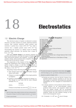
  • 1. 18.1 Electric Charge The electrical nature of matter is inherent in atomic structure. An atom consists of a small, relatively massive nucleus that contains particles called protons and neutrons. A proton has a mass 1.673´ - 10 27 kg, while a neutron has a slightly greater mass 1.675 10 kg.–27 ´ Surrounding the nucleus is a diffuse cloud of orbiting particles called electrons. An electron has a mass of 9.11 10 kg31 ´ - . Like mass electric charge is an intrinsic property of protons and electrons, and only two types of charge have been discovered positive and negative. A proton has a positive charge, and an electron has a negative charge. A neutron has no net electric charge. The magnitude of the charge on the proton exactly equals the magnitude of the charge on the electron. The proton carries a charge +e and the electron carries a charge -e. The SI unit of charge is Coulomb( )C and e has the value, e = ´ - 1.6 10 C19 Regarding charge following points are worth noting: 1. Like charges repel each other and unlike charges attract each other. 2. Charge is a scalar and can be of two types positive or negative. 3. Charge is quantized. The quantum of charge is e. The charge on any body will be some integral multiple of e, i.e., q ne= ± where, n = ¼1 2 3, , Charge on any body can never be 1 3 e æ è ç ö ø ÷ ,1.5e, etc. Note 1. Apart from charge, energy, angular momentum and mass are also quantized. The quantum of energy is hnand that of angular momentum is h 2p . Quantum of mass is yet not known. 2. The protons and neutrons are combination of other entities called quarks, which have charges 1 3 e and ± 2 3 e. However, isolated quarks have not been observed, so, quantum of charge is still e. 4. During any process, the net electric charge of an isolated system remains constant or we can say that charge is conserved. Pair production and pair annihilation are two examples of conservation of charge. 5. A charge particle at rest produces electric field. A charge particle in an unaccelerated motion produces both electric and magnetic fields but does not radiate energy. But an accelerated charged particle not only produces an electric and magnetic fields but also radiates energy in the form of electromagnetic waves. 6. 1 Coulomb = ´ =3 109 esu 1 10 emu of charge. 18 Electrostatics Chapter Snapshot q Electric Charge q Conductors and Insulators q Charging of a Body q Coulomb’s Law q Electric Field q Electric Potential Energy q Electric Potential q Relation between Electric Field and Potential q Equipotential Surfaces q Electric Dipole q Gauss’s Law q Properties of a Conductor q Electric Field and Potential due to Charged Spherical Shell of Solid Conducting Sphere q Electric Field and Potential due to a Solid Sphere of Charge q Capacitance Get Discount Coupons for your Coaching institute and FREE Study Material at www.PICKMYCOACHING.com Get Discount Coupons for your Coaching institute and FREE Study Material at www.PICKMYCOACHING.com1 www.pickM yCoaching.com
  • 2. Example 18.1 How many electrons are there in one coulomb of negative charge? Solution The negative charge is due to the presence of excess electrons, since they carry negative charge. Because an electron has a charge whose magnitude is e = ´ - 1.6 10 C19 , the number of electrons is equal to the charge qdivided by the charge e on each electron. Therefore, the number n of electrons is n q e = = ´ - 1.0 1.6 10 19 = ´6.25 1018 18.2 Conductors and Insulators For the purpose of electrostatic theory all substances can be divided into two main groups — conductors and insulators. In conductors electric charges are free to move from one place to another, whereas in insulators they are tightly bound to their respective atoms. In an uncharged body there are equal number of positive and negative charges. The examples of conductors of electricity are the metals, human body and the earth and that of insulators are glass, hard rubber and plastics. In metals, the free charges are free electrons known as conduction electrons. Semiconductors are a third class of materials, and their electrical properties are somewhere between those of insulators and conductors. Silicon and germanium are well known examples of semiconductors. 18.3 Charging of a Body Mainly there are following three methods of charging a body: (i) Charging by Rubbing The simplest way to experience electric charges is to rub certain bodies against each other. When a glass rod is rubbed with a silk cloth the glass rod acquires some positive charge and the silk cloth acquires negative charge by the same amount. The explanation of appearance of electric charge on rubbing is simple. All material bodies contain large number of electrons and equal number of protons in their normal state. When rubbed against each other, some electrons from one body pass onto the other body. The body that donates the electrons becomes positively charged while that which receives the electrons becomes negatively charged. For example when glass rod is rubbed with silk cloth, glass rod becomes positively charged because it donates the electrons while the silk cloth becomes negatively charged because it receives electrons. Electricity so obtained by rubbing two objects is also known as frictional electricity. The other places where the frictional electricity can be observed are when amber is rubbed with wool or a comb is passed through a dry hair. Clouds also become charged by friction. (ii) Charging by Contact When a negatively charged ebonite rod is rubbed on a metal object, such as a sphere, some of the excess electrons from the rod are transferred to the sphere. Once the electrons are on the metal sphere, where they can move readily, they repel one another and spread out over the sphere’s surface. The insulated stand prevents them from flowing to the earth. When the rod is removed the sphere is left with a negative charge distributed over its surface. In a similar manner the sphere will be left with a positive charge after being rubbed with a positively charged rod. In this case, electrons from the sphere would be transferred to the rod. The process of giving one object a net electric charge by placing it in contact with another object that is already charged is known as charging by contact. (iii) Charging by Induction It is also possible to charge a conductor in a way that does not involve contact. In Fig. (a) a negatively charged rod brought close to (but does not touch) a metal sphere. In the sphere, the free electrons close to the rod move to the other side (by repulsion). As a result, the part of the sphere nearer to the rod becomes positively charged and the part farthest from the rod negatively charged. This phenomenon is called induction. Now if the rod is removed, the free electrons return to their original places and the charged regions disappear. Under most conditions the earth is a 2 Objective Physics Volume 2 –––––––– –––––––– – ––––– – – – – – –– – – – – – – – –––– – – Ebonite rod Metal sphere Insulated stand Fig. 18.1 –––––––– –––––––– Ebonite rod Metal sphere Insulated stand (a) (b) + ++ ––– + + + + + ++ – – – – –– + ++ ––– + + + + + ++ – – – – –– Grounding wire –––––––– –––––––– (c) + + + + + + + + + + + ++ + + + + ++ Earth Fig. 18.2 – – – – – – + – Plastic Ebonite rod + – + – + – + – Fig. 18.3 Get Discount Coupons for your Coaching institute and FREE Study Material at www.PICKMYCOACHING.com Get Discount Coupons for your Coaching institute and FREE Study Material at www.PICKMYCOACHING.com2 www.pickM yCoaching.com
  • 3. good electric conductor. So when a metal wire is attached between the sphere and the ground as in Fig. (b) some of the free electrons leave the sphere and distribute themselves on the much larger earth. If the grounding wire is then removed, followed by the ebonite rod, the sphere is left with a net positive charge. The process of giving one object a net electric charge without touching the object to a second charged object is called charging by induction. The process could also be used to give the sphere a net negative charge, if a positively charged rod were used. Then, electrons would be drawn up from the ground through the grounding wire and onto the sphere. If the sphere were made from an insulating material like plastic, instead of metal, the method of producing a net charge by induction would not work, because very little charge would flow through the insulating material and down the grounding wire. However, the electric force of the charged rod would have some effect as shown in figure. The electric force would cause the positive and negative charges in the molecules of the insulating material to separate slightly, with the negative charges being pushed away from the negative rod. The surface of the plastic sphere does acquire a slight induced positive charge, although no net charge is created. Example 18.2 If we comb our hair on a dry day and bring the comb near small pieces of paper, the comb attracts the pieces, why? Solution This is an example of frictional electricity and induction. When we comb our hair it gets positively charged by rubbing. When the comb is brought near the pieces of paper some of the electrons accumulate at the edge of the paper piece which is closer to the comb. At the farther end of the piece there is deficiency of electrons and hence, positive charge appears there. Such a redistribution of charge in a material, due to presence of a nearby charged body is called induction. The comb exerts larger attraction on the negative charges of the paper piece as compared to the repulsion on the positive charge. This is because the negative charges are closer to the comb. Hence, there is a net attraction between the comb and the paper piece. Example 18.3 Does the attraction between the comb and the piece of papers last for longer period of time? Solution No, because the comb loses its net charge after some time. The excess charge of the comb transfers to earth through our body after some time. Example 18.4 Can two similarly charged bodies attract each other? Solution Yes, when the charge on one body ( )q1 is much greater than that on the other( )q2 and they are close enough to each other so that force of attraction between q1 and induced charge on the other exceeds the force of repulsion between q1 and q2 . However two similar point charges can never attract each other because no induction will take place here. Example 18.5 Does in charging the mass of a body change? Solution Yes, as charging a body means addition or removal of electrons and electron has a mass. Example 18.6 Why a third hole in a socket provided for grounding? Solution All electric appliances may end with some charge due to faulty connections. In such a situation charge will be accumulated on the appliance. When the user touches the appliance he may get a shock. By providing the third hole for grounding all accumulated charge is discharged to the ground and the appliance is safe. 18.4 Coulomb’s Law The law that describes how charges interact with one another was discovered by Charles Augustin de Coulomb in 1785. With a sensitive torsion balance, Coulomb measured the electric force between charged spheres. In Coulomb’s experiment the charged spheres were much smaller than the distance between them so that the charges could be treated as point charges. The results of the experiments of Coulomb and others are summarized in Coulomb’s law. The electric force Fe exerted by one point charge on another acts along the line between the charges. It varies inversely as the square of the distance separating the charges and is proportional to the product of charges. The force is repulsive if the charges have the same sign and attractive if the charges have opposite signs. The magnitude of the electric force exerted by a charge q1 on another charge q2 a distance r away is thus, given by F k q q r e = | |1 2 2 …(i) The value of the proportionality constant k in Coulomb’s law depends on the system of units used. In SI units the constant k is, k 8.987551787 10 N-m C 9 2 2 = ´ » ´8.988 10 N-m C 9 2 2 The value of k is known to such a large number of significant digits because this value is closely related to the speed of light in vacuum. This speed is defined to be exactly c 2.99792458 10 m / s8 = ´ . The numerical value of k is defined in terms of c to be precisely. k c= æ è ç ç ö ø ÷ ÷ - 10 7 2 2 2N s C - This constant k is often written as 1 4 0pe , where e0 (epsilon-nought) is another constant. This appears to complicate matters, but it actually simplifies many formulae that we will encounter in later chapters. Thus, Eq. (i) can be written as, F q q r e = 1 4 0 1 2 2 pe | | …(ii) Chapter 18 · Electrostatics 3 Get Discount Coupons for your Coaching institute and FREE Study Material at www.PICKMYCOACHING.com Get Discount Coupons for your Coaching institute and FREE Study Material at www.PICKMYCOACHING.com3 www.pickM yCoaching.com
  • 4. Here, 1 4 0pe 10 N - s C 7 2 2 2 = æ è ç ç ö ø ÷ ÷ - c Substituting value of c 2.99792458 10 m / s8 = ´ , we get 1 4 0p e = ´8.99 10 N - m /C9 2 2 In examples and problems we will often use the approximate value, 1 4 0pe 9.0 10 N - m /C9 2 2 = ´ Here, the quantity e0 is called the permittivity of free space. It has the value, e0 = ´8.854 10 C /N - m–12 2 2 Regarding Coulomb’s law following points are worth noting: (1) Coulomb’s law stated above describes the interaction of two point charges. When two charges exert forces simultaneously on a third charge, the total force acting on that charge is the vector sum of the forces that the two charges would exert individually. This important property, called the principle of superposition of forces, holds for any number of charges. Thus, F F F Fnet = + + ¼+1 2 n (2) The electric force is an action reaction pair, i.e., the two charges exert equal and opposite forces on each other. (3) The electric force is conservative in nature. (4) Coulomb’s law as we have stated above can be used for point charges in vacuum. If some dielectric (insulator) is present in the space between the charges, the net force acting on each charge is altered because charges are induced in the molecules of the intervening medium. We will describe this effect later. Here at this moment it is enough to say that the force decreases K times if the medium extends till infinity. Here K is a dimensionless constant which depends on the medium and called dielectric constant of the medium. Thus, F q q r e = × 1 4 0 1 2 2 pe (in vacuum) F F K K q q r e e ¢ = = × 1 4 0 1 2 2 pe = × 1 4 1 2 2 pe q q r (in medium) Here, e e= 0K is called permittivity of the medium. Objective Galaxy 1 8 . 1 1. In few problems of electrostatics Lami’s theorem is very useful. According to this theorem, ‘if three concurrent forces F F1 2, and F3 as shown in figure are in equilibrium or if F F F1 2 2 0+ + = , then F F F1 2 3 sin sin sina b g = = 2. Suppose the position vectors of two charges q1 and q2 are r1 and r2 , then, electric force on charge q1 due to charge q2 is, F r r r r1 0 1 2 1 2 3 1 1 1 4 = × pe q q | – | ( – ) Similarly, electric force on q2 due to charge q1 is F r r r r2 0 1 2 2 1 3 2 1 1 4 = × pe q q | – | ( – ) Here q1 and q2 are to be substituted with sign. r i j k1 1 1 1= + +x y z$ $ $ and r i j k2 2 2 2= + +x y z$ $ $ where ( , , )x y z1 1 1 and ( , , )x y z2 2 2 are the co-ordinates of charges q1 and q2. Example 18.7 What is the smallest electric force between two charges placed at a distance of 1.0 m. Solution F q q r e = × 1 4 0 1 2 2 pe …(i) For Fe to be minimum q q1 2 should be minimum. We know that ( ) ( )min minq q1 2= = e = ´ - 1.6 10 C19 Substituting in Eq. (i), we have ( )minFe = ´ ´ ´- - (9.0 10 ) (1.6 10 ) (1.6 10 ) (1. 9 19 19 0)2 = ´ - 2.304 10 N28 Example 18.8 Three charges q C1 1= m , q C2 2= – m and q C3 3= m are placed on the vertices of an equilateral triangle of side 1.0 m. Find the net electric force acting on charge q1. 4 Objective Physics Volume 2 a b g F1 F2 F3 Fig. 18.5 Fe q1 q2 Fe In vacuum r Fig. 18.4 Get Discount Coupons for your Coaching institute and FREE Study Material at www.PICKMYCOACHING.com Get Discount Coupons for your Coaching institute and FREE Study Material at www.PICKMYCOACHING.com4 www.pickM yCoaching.com
  • 5. How to Proceed Charge q2 will attract charge q1 (along the line joining them) and charge q3 will repel charge q1. Therefore, two forces will act on q1, one due to q2 and another due to q3 . Since, the force is a vector quantity both of these forces (say F1 andF2 ) will be added by vector method. Following are two methods of their addition. Solution Method 1. In the figure, | |F1 1 0 1 2 2 1 4 = = ×F q q rpe = magnitude of force between andq q1 2 = ´ ´ ´- - (9.0 10 ) (1.0 10 ) (2.0 10 ) (1.0) 9 6 6 2 = ´ - 1.8 10 N2 Similarly, | |F2 2 0 1 3 2 1 4 = = ×F q q rpe = magnitude of force between andq q1 2 = ´ ´ ´- - (9.0 10 ) (1.0 10 ) (3.0 10 ) (1.0) 9 6 6 2 = ´ - 2.7 10 N2 Now, | | cosFnet = + + °F F F F1 2 2 2 1 22 120 = + + æ è ç ö ø ÷ æ è ç ç ö ø ÷ ÷ (1.8) (2.7) 2 (1.8) (2.7) – 1 2 2 2 ´ - 10 N2 = ´ - 2.38 10 N2 and tan sin cos a = ° + ° F F F 2 1 2 120 120 = ´ ´ + ´ - - - - (2.7 10 ) (0.87) (1.8 10 ) (2.7 10 ) 2 2 2 1 2 æ è ç ö ø ÷ or a = °79.2 Thus, the net force on charge q1 is 2.38 10 N2 ´ - at an angle a = °79.2 with a line joining q1 and q2 as shown in the figure. Method 2. In this method let us assume a co-ordinate axes with q1 at origin as shown in figure. The co-ordinates of q q1 2, and q3 in this co-ordinate system are (0, 0, 0), (1 m, 0, 0) and (0.5 m, 0.87 m, 0) respectively. Now, F1 1 2= force on due to chargeq q = × 1 4 0 1 2 1 2 3 1 2 pe q q | – | ( – ) r r r r = ´ ´ ´(9.0 10 ) (1.0 10 ) (–2.0 10 ) (1.0) 9 –6 –6 3 ´ + +[( – ) $ ( – ) $ ( – ) $ ]0 1 0 0 0 0i j k = ´ - (1.8 10 2 $)i N and F2 = force on due to charge1 3q q = × 1 4 0 1 3 1 3 3 1 3 pe q q | – | ( – ) r r r r = ´ ´ ´(9.0 10 ) (1.0 10 ) (3.0 10 ) (1.0) 9 –6 –6 3 ´ + +[( – $ ( – ) $ ( – ) $]0 0 0 00.5) 0.87i j k = ´ - ( – $ – $)1.35 2.349i j 10 2 N Therefore, net force on q1 is, F F F= +1 2 = ´( $ $ – 0.45 – 2.349 ) 10i j 2 N Note Once you write a vector in terms of $, $i j and $k, there is no need of writing the magnitude and direction of vector separately. Example 18.9 Two identical balls each having a density r are suspended from a common point by two insulating strings of equal length. Both the balls have equal mass and charge. In equilibrium each string makes an angle q with vertical. Now, both the balls are immersed in a liquid. As a result the angle q does not change. The density of the liquid is s. Find the dielectric constant of the liquid. Solution Each ball is in equilibrium under the following three forces: (i) tension (ii) electric force and (iii) weight So, Lami’s theorem can be applied. Chapter 18 · Electrostatics 5 q1 q2 q3 Fig. 18.6 q1 q2 q3 a 120° F1 F2 Fnet Fig. 18.7 q1 q2 q3y x Fig. 18.8 In vacuum Fe q q w T In liquid Fe¢ q q w ¢ T ¢ Fig. 18.9 Get Discount Coupons for your Coaching institute and FREE Study Material at www.PICKMYCOACHING.com Get Discount Coupons for your Coaching institute and FREE Study Material at www.PICKMYCOACHING.com5 www.pickM yCoaching.com
  • 6. In the liquid, F F K e e ¢ = where, K = dielectric constant of liquid and w w¢ = - upthrust Applying Lami’s theorem in vacuum w Fe sin ( ) sin ( )90 180° + = ° -q q or w Fe cos sinq q = …(i) Similarly in liquid, w Fe¢ = ¢ cos sinq q …(ii) Dividing Eq. (i) by Eq. (ii), we get w w F F e e ¢ = ¢ or K w w = – upthrust as F F Ke e¢ = æ è ç ç ö ø ÷ ÷ = V g V g V g r r s– (V = volume of ball) or K = - r r s Note In the liquid Fe and w have been changed. Therefore, T will also change. 18.5 Electric Field A charged particle cannot directly interact with another particle kept at a distance. A charge produces something called an electric field in the space around it and this electric field exerts a force on any other charge (except the source charge itself) placed in it. Thus, the region surrounding a charge or distribution of charge in which its electrical effects can be observed is called the electric field of the charge or distribution of charge. Electric field at a point can be defined in terms of either a vector function E called electric field strength or a scalar function V called electric potential. The electric field can also be visualised graphically in terms of lines of force. Electric Field Strength ( )E Like its gravitational counterpart, the electric field strength (often called electric field) at a point in an electric field is defined as the electrostatic forceFe per unit positive charge. Thus, if the electrostatic force experienced by a small test charge q0 isFe, then field strength at that point is defined as, E F = ® lim q e q0 0 0 The electric field is a vector quantity and its direction is the same as the direction of the forceFe on a positive test charge. The SI unit of electric field is N/C. Here, it should be noted that the test charge q0 does not disturb other charges which produces E. With the concept of electric field, our description of electric interactions has two parts. First, a given charge distribution acts as a source of electric field. Second, the electric field exerts a force on any charge that is present in this field. An Electric Field Leads to a Force Suppose there is an electric field strength E at some point in an electric field, then the electrostatic force acting on a charge +q is qE in the direction of E, while on the charge – q it is qE in the opposite direction of E. Example 18.10 An electric field of 105 N/C points due west at a certain spot. What are the magnitude and direction of the force that acts on a charge of + 2 mC and - 5 mC at this spot? Solution Force on + =2 mC qE = ´( )( )– 2 10 106 5 = 0.2N (due west) Force on – C5 m = ´(5 10 ) (10 )–6 5 = 0.5 N (due east) Electric Field Due to a Point Charge The electric field produced by a point charge q can be obtained in general terms from Coulomb’s law. First note that the magnitude of the force exerted by the charge q on a test charge q0 is, F qq r e = × 1 4 0 0 2 p e then divide this value by q0 to obtain the magnitude of the field. E q r = × 1 4 0 2 pe If q is positive E is directed away from q. On the other hand if q is negative, then E is directed towards q. The electric field at a point is a vector quantity. Suppose E1 is the field at a point due to a charge q1 and E2 is the field at the same point due to a charge q2. The resultant field when both the charges are present is E E E= +1 2 6 Objective Physics Volume 2 + r q0 Fe q + Eq –q E Fig. 18.10 Get Discount Coupons for your Coaching institute and FREE Study Material at www.PICKMYCOACHING.com Get Discount Coupons for your Coaching institute and FREE Study Material at www.PICKMYCOACHING.com6 www.pickM yCoaching.com
  • 7. If the given charge distribution is continuous, we can use the technique of integration to find the resultant electric field at a point. Example 18.11 Two positive point charges q C1 16= m and q C2 4= m , are separated in vacuum by a distance of 3.0 m. Find the point on the line between the charges where the net electric field is zero. Solution Between the charges the two field contributions have opposite directions, and the net electric field is zero at a point (say P), where the magnitudes of E1 and E2 are equal. However, since, q q2 1< , point P must be closer to q2 , in order that the field of the smaller charge can balance the field of the larger charge. At P, E E1 2= or 1 4 1 40 1 1 2 0 2 2 2 pe pe q r q r = × r r q q 1 2 1 2 = = = 16 4 2 …(i) Also, r r1 2+ = 3.0 m …(ii) Solving these equations, we get r1 2 m= and r2 1 m= Thus, the point P is at a distance of 2 m from q1 and 1 m from q2 . Electric Field of a Ring of Charge Electric field at distance x from the centre of uniformly charged ring of total charge q on its axis is given by, E qx x R x = æ è çç ö ø ÷÷ + 1 4 0 2 2 3 2 pe ( ) / Direction of this electric field is along the axis and away from the ring in case of positively charged ring and towards the ring in case of negatively charged ring. From the above expression, we can see that (i) Ex = 0 at x = 0, i.e., field is zero at the centre of the ring. We should expect this, charges on opposite sides of the ring would push in opposite directions on a test charge at the centre, and the forces would add to zero. (ii) E q x x = × 1 4 0 2 pe for x R>> , i.e., when the point P is much farther from the ring, its field is the same as that of a point charge. To an observer far from the ring, the ring would appear like a point, and the electric field reflects this. (iii) Ex will be maximum where dE dx x = 0. Differentiating Ex w.r.t. x and putting it equal to zero, we get x R = 2 and Emax comes out to be, 2 3 1 43 0 2 pe × æ è çç ö ø ÷÷ q R . Electric Field of an Infinitely Long Line Charge Electric field at distance r from an infinitely long line charge is given by E r = l pe2 0 Here l is charge per unit length. Direction of this electric field is away from the line charge in case of positively charged line charge and towards the line charge in case of negatively charged line charge. or E r µ 1 Thus, E-r graph is as shown in Fig. 18.15. The direction of E is radially outward from the line. Chapter 18 · Electrostatics 7 + + + + + + + + + + + + Ex P Exx x R R Fig. 18.12 R 2 Ex Emax x Fig. 18.13 + + + + + + + + + + + + + + + + + + E l l r P P Er Fig. 18.14 E r Fig. 18.15 + PE2 q1 + E1 q2 r1 r2 Fig. 18.11 Get Discount Coupons for your Coaching institute and FREE Study Material at www.PICKMYCOACHING.com Get Discount Coupons for your Coaching institute and FREE Study Material at www.PICKMYCOACHING.com7 www.pickM yCoaching.com
  • 8. Example 18.12 A charge q C=1m is placed at point ( , , )1 2 4m m m. Find the electric field at point P m m m( , – , )0 4 3 . Solution Here, rq = + +$ $ $i j k2 4 and rp = +– $ $4 3j k r rp q– – $ – $ – $= i j k6 or | – | (– ) (– ) (– )r rp q = + +1 6 12 2 2 = 38 m Now, E = × 1 4 0 3 pe q p q p q | – | ( – ) r r r r Substituting the values, we have E i j k= ´ ´( )( ) ( ) (–$ – $ – $) – / 9.0 1.010 10 38 6 9 6 3 2 = ( $ $ $)–38.42 – 230.52 – 38.42i j k N C Electric Field Lines As we have seen, electric charges create an electric field in the space surrounding them. It is useful to have a kind of map that gives the direction and indicates the strength of the field at various places. Field lines, a concept introduced by Michael Faraday, provide us with an easy way to visualize the electric field. “An electric field line is an imaginary line or curve drawn through a region of space so that its tangent at any point is in the direction of the electric field vector at that point. The relative closeness of the lines at some place give an idea about the intensity of electric field at that point.” The electric field lines have the following properties: 1. The tangent to a line at any point gives the direction of E at that point. This is also the path on which a positive test charge will tend to move if free to do so. 2. Electric field lines always begin on a positive charge and end on a negative charge and do not start or stop in midspace. 3. The number of lines leaving a positive charge or entering a negative charge is proportional to the magnitude of the charge. This means, for example that if 100 lines are drawn leaving a + 4 mC charge then 75 lines would have to end on a –3 mCcharge. 4. Two lines can never intersect. If it happens then two tangents can be drawn at their point of intersection, i.e., intensity at that point will have two directions which is absurd. 8 Objective Physics Volume 2 EQ Ep P Q A | | | |E EA B> B Fig. 18.16 Objective Galaxy 1 8 . 2 1. Suppose a charge q is placed at a point whose position vector is rq and we want to find the electric field at a point P whose position vector is rp Then in vector form the electric field is given by, E r r r r= × 1 4 0 3 pe q p q p q | – | ( – ) Here, r i j zp p p px y z= + +$ $ $ and r i j kq q q qx y z= + +$ $ $ q –q (a) (b) (c) + – q q + (d) +qq – (e) –q –q + q2q – (f) Fig. 18.17 Get Discount Coupons for your Coaching institute and FREE Study Material at www.PICKMYCOACHING.com Get Discount Coupons for your Coaching institute and FREE Study Material at www.PICKMYCOACHING.com8 www.pickM yCoaching.com
  • 9. 5. In a uniform field, the field lines are straight parallel and uniformly spaced. 6. The electric field lines can never form closed loops as a line can never start and end on the same charge. 7. Electric field lines also give us an indication of the equipotential surface (surface which has the same potential) 8. Electric field lines always flow from higher potential to lower potential. 9. In a region where there is no electric field, lines are absent. This is why inside a conductor (where electric field is zero) there, cannot be any electric field line. 10. Electric lines of force ends or starts normally from the surface of a conductor. 18.6 Electric Potential Energy If the force F is conservative, the work done by F can always be expressed in terms of a potential energy U. When the particle moves from a point where the potential energy is Ua to a point where it is Ub, the change in potential energy is, DU U Ub a= – . This is related by the work Wa b® as W U U U U Ua b a b b a® = = =– – ( – ) – D …(i) Here Wa b® is the work done in displacing the particle from a to b by the conservative force (here electrostatic) not by us. Moreover we can see from Eq. (i) that if Wa b® is positive, DU is negative and the potential energy decreases. So, whenever the work done by a conservative force is positive, the potential energy of the system decreases and vice versa. That’s what happens when a particle is thrown upwards, the work done by gravity is negative, and the potential energy increases. Example 18.13 A uniform electric field E0 is directed along positive y-direction. Find the change in electric potential energy of a positive test charge q0 when it is displaced in this field from y ai = to y af = 2 along the y-axis. Solution Electrostatic force on the test charge, F q Ee = 0 0 (along positive y-direction) W Ui f- = – D or DU Wi f= -– = – [ ( – )]q E a a0 0 2 = – q E a0 0 Note Here work done by electrostatic force is positive. Hence, the potential energy is decreasing. Electric Potential Energy of Two Charges The idea of electric potential energy is not restricted to the special case of a uniform electric field as in example 18.13. Let us now calculate the work done on a test charge q0 moving in a non-uniform electric field caused by a single, stationary point charge q. The Coulomb’s force on q0 at a distance r from a fixed charge q is, F qq r = × 1 4 0 0 2 pe If the two charges have same signs, the force is repulsive and if the two charges have opposite signs, the force is attractive. The force is not constant during the displacement, so we have to integrate to calculate the work Wa b® done on q0 by this force as q0 moves from a to b. W F dra b r r a b ® = ò = ×ò 1 4 0 0 2 per r a b qq r dr = æ è çç ö ø ÷÷ qq r ra b 0 04 1 1 pe – Being a conservative force this work is path independent. From the definition of potential energy, U U Wb a a b– –= - = æ è çç ö ø ÷÷ qq r rb a 0 04 1 1 pe – We choose the potential energy of the two charge system to be zero when they have infinite separation. This meansU¥ = 0. The potential energy when the separation is r is Ur U U qq r r – –¥ = ¥ æ è ç ö ø ÷0 04 1 1 pe or U qq r r = 0 04 1 pe This is the expression for electric potential energy of two point charges kept at a separation r. In this expression both the charges q and q0 are to be substituted with sign. Electric Potential Energy of a System of Charges To find electrical potential energy of a system of charges, we make pairs. If there are total n charges then total number of pairs are n n( ) . -1 2 Neither of the pair should be repeted, nor should be left. Chapter 18 · Electrostatics 9 E0 q E0 0 + q0 Fig. 18.18 q a q0 b r ra rb Fig. 18.19 Get Discount Coupons for your Coaching institute and FREE Study Material at www.PICKMYCOACHING.com Get Discount Coupons for your Coaching institute and FREE Study Material at www.PICKMYCOACHING.com9 www.pickM yCoaching.com
  • 10. For example electric potential energy of four point charges q q q1 2 3, , and q4 would be given by, U q q r q q r q q r q q r q q r q q = + + + + + 1 4 0 4 3 43 4 2 42 4 1 41 3 2 32 3 1 31 2 pe 1 21r é ë ê ù û ú …(ii) Here, all the charges are to be substituted with sign. Example 18.14 Four charges q C1 1= m , q C2 2= m , q C3 3= – m and q C4 4= m are kept on the vertices of a square of side 1 m. Find the electric potential energy of this system of charges. Solution In this problem, r r r r41 43 32 21 1= = = = m and r r42 31 2 2 1 1 2= = + =( ) ( ) m Substituting the proper values with sign in Eq. (ii), we get U = ´( )( )( )– – 9.0 10 10 109 6 6 (4)(–3) 1 (4)(2) 2 (4)(1) 1 (–3)(2) 1 (–3)(1) 2 + + + + (2)(1) 1 + é ëê ù ûú = ´ + é ëê ù ûú(9.0 10 12 5 2 3– ) – = ´– 7.62 10 J–2 Note Here negative sign of U implies that positive work has been done by electrostaticforcesinassemblingthesechargesatrespectivedistancesfrominfinity. Example 18.15 Two point charges are located on the x-axis, q C1 1= – m at x = 0 and q C2 1= + m at x m=1 . (a) Find the work that must be done by an external force to bring a third point charge q C3 1= + m from infinity to x m= 2 . (b) Find the total potential energy of the system of three charges. Solution (a) The work that must be done on q3 by an external force is equal to the difference of potential energy U when the charge is at x = 2 m and the potential energy when it is at infinity. W U Uf i= – = + + é ë ê ù û ú 1 4 0 3 2 32 3 1 31 2 1 21pe q q r q q r q q rf f f( ) ( ) ( ) – ( ) ( ) ( ) 1 4 0 3 2 32 3 1 31 2 1 21pe q q r q q r q q ri i i + + é ë ê ù û ú Here, ( ) ( )r ri f21 21= and ( ) ( )r ri i32 31= = ¥ W q q r q q rf f = + é ë ê ù û ú 1 4 0 3 2 32 3 1 31pe ( ) ( ) Substituting the values, we have W = ´ +(9.0 10 ) (10 ) (1) (1) (1.0) (1) (–1) (2.0 9 –12 ) é ë ê ù û ú = ´4.5 10 J–3 (b) The total potential energy of the three charges is given by, U q q r q q r q q r = + + æ è çç ö ø ÷÷ 1 4 0 3 2 32 3 1 31 2 1 21pe = ´ + +(9.0 10 ) (1) (1) (1.0) (1) (–1) (2.0) (1) (9 –1) (1.0) (1 é ë ê ù û ú 0 12– ) = ´– 4.5 10–3 J Example 18.16 Two point charges q q C1 2 2= = m are fixed at x m1 3= + and x m2 3= – as shown in figure. A third particle of mass 1 g and charge q C3 4= – m are released from rest at y m= 4.0 . Find the speed of the particle as it reaches the origin. How to Proceed Here the charge q3 is attracted towards q1 and q2 both. So, the net force on q3 is towards origin. By this force charge is accelerated towards origin, but this acceleration is not constant. So, to obtain the speed of particle at origin by kinematics, we will have to find first the acceleration at same intermediate position and then will have to integrate it with proper limits. On the other hand it is easy to use energy conservation principle as the only forces are conservative. 10 Objective Physics Volume 2 1 m 1 m q1 q2 q3q4 Fig. 18.20 y x q2 q1 x1 = 3 mx2 = –3 m O q3 y = 4 m Fig. 18.21 y x q2 q1 O q3 Fnet Fig. 18.22 q2 q3 q1 q4 Get Discount Coupons for your Coaching institute and FREE Study Material at www.PICKMYCOACHING.com Get Discount Coupons for your Coaching institute and FREE Study Material at www.PICKMYCOACHING.com10 www.pickM yCoaching.com
  • 11. Solution Let v be the speed of particle at origin. From conservation of mechanical energy, U K U Ki i f f+ = + or 1 4 0 0 3 2 32 3 1 31 2 1 21pe q q r q q r q q ri i i( ) ( ) ( ) + + é ë ê ù û ú + = + + é ë ê ù û ú + 1 4 1 20 3 2 32 3 1 31 2 1 21 2 pe q q r q q r q q r mv f f f( ) ( ) ( ) Here, ( ) ( )r ri f21 21= Substituting the proper values, we have (9.0 10 ) (– 4) (2) (5.0) (– 4) (2) (5.0) 9 ´ + é ë ê ù û ú ´ 10–12 = ´ + é ë ê ù û ú(9.0 10 ) (– 4) (2) (3.0) (– 4) (2) (3.0) 9 10 1 2 10–12 –3 ´ + ´ ´ v2 ( ) – ( ) –– – – 9 10 16 5 9 10 16 3 1 2 103 3 3 2 ´ æ è ç ö ø ÷ = ´ æ è ç ö ø ÷ + ´ ´ v ( )( )– – 9 10 16 2 15 1 2 103 3 2 ´ æ è ç ö ø ÷ = ´ ´ v v = 6.2 m s/ 18.7 Electric Potential As we have discussed in Article 18.5 that an electric field at any point can be defined in two different ways: (i) by the field strength E, and (ii) by the electric potential V at the point under consideration. Both E and V are functions of position and there is a fixed relationship between these two. Of these, the field strengthEis a vector quantity while the electric potential V is a scalar quantity. In this article we will discuss about the electric potential and in the next the relationship between E and V. Potential is the potential energy per unit charge. Electric potential at any point in an electric field is defined as the potential energy per unit charge, same as the field strength is defined as the force per unit charge. Thus, V U q = 0 or U q V= 0 The SI unit of potential is volt ( V ) which is equal to joule per coulomb. So, 1 V 1 volt 1 J /C 1 joule / coulomb= = = The work done by the electrostatic force in displacing a test charge q0 from a to b in an electric field is defined as the negative of change in potential energy between them, or DU Wa b= – – U U Wb a a b– – –= We divide this equation by q0, U q U q W q b a a b 0 0 0 - = – – or V V W q a b a b – – = 0 as V U q = 0 Thus, the work done per unit charge by the electric force when a charged body moves from a to b is equal to the potential at a minus the potential at b. We sometimes abbreviate this difference as V V Vab a b= – . Another way to interpret the potential difference Vab is that the potential at a minus potential at b, equals the work that must be done to move a unit positive charge slowly from b to a against the electric force. V V W q a b b a – ( )– = external force 0 Absolute Potential at Some Points Suppose we take the point b at infinity and as a reference point assign the value Vb = 0, the above equations can be written as V V W q W q a b a b b a – ( ) ( )– – = = electric force external force 0 0 or V W q W q a a a = = ¥ ¥( ) ( )– –electric force external force 0 0 Thus, the absolute electric potential at point a in an electric field can be defined as the work done in displacing a unit positive charge from infinity to a by the external force or the work done per unit positive charge in displacing it from a to infinity. Objective Galaxy 1 8 . 3 Following three formulae are very useful in the problems related to work done in electric field. ( ) ( – )–W q V Va b a belectric force = 0 ( ) ( – ) – ( )– –W q V V Wa b b a a bexternal force electric force= =0 ( )–W q Va a¥ =external force 0 Here, q Va0, andVb are to be substituted with sign. Example 18.17 The electric potential at point A is 20 V and at B is – 40 V. Find the work done by an external force and electrostatic force in moving an electron slowly from B to A. Solution Here, the test charge is an electron, i.e., q0 – 1.6 10 C–19 = ´ VA = 20 V and VB = – 40 V Work done by external force ( ) ( – )–W q V VB A A Bexternal force = 0 Chapter 18 · Electrostatics 11 Get Discount Coupons for your Coaching institute and FREE Study Material at www.PICKMYCOACHING.com Get Discount Coupons for your Coaching institute and FREE Study Material at www.PICKMYCOACHING.com11 www.pickM yCoaching.com
  • 12. = ´(– 1.6 10 ) [(20) – (– 40)]–19 = ´– 9.6 10 J–18 Work done by electric force ( ) – ( )– –W WB A B Aelectric force external force= = ´– (– 9.6 10 J)–18 = ´9.6 10 J–18 Note Here we can see that the electron (a negative charge) moves from B (lower potential) to A (higher potential) and the work done by electric force is positive. Therefore, we may conclude that whenever a negative charge moves from a lower potential to higher potential work done by the electric force is positive or when a positive charge moves from lower potential to higher potential the work done by the electric force is negative. Example 18.18 Find the work done by some external force in moving a charge q C= 2 m from infinity to a point where electric potential is104 V. Solution Using the relation, ( )–W qVa a¥ =external force We have, ( ) ( )( )– – W a¥ = ´external force 2 10 106 4 = ´2 10 2– J Electric Potential Due to a Point Charge q From the definition of potential, V U q = 0 = × 1 4 0 0 0 pe q q r q or V q r = × 1 4 0pe Here, r is the distance from the point charge q to the point at which the potential is evaluated. If q is positive, the potential that it produces is positive at all points; if q is negative, it produces a potential that is negative everywhere. In either case, V is equal to zero at r = ¥. Electric Potential Due to a System of Charges Just as the electric field due to a collection of point charges is the vector sum of the fields produced by each charge, the electric potential due to a collection of point charges is the scalar sum of the potentials due to each charge. V q r i ii = å 1 4 0pe Objective Galaxy 1 8 . 4 In the equationV q r i ii = å 1 4 0pe if the whole charge is at equal distance r0 from the point where V is to be evaluated, then we can write, V q r = × 1 4 0 0pe net where qnet is the algebraic sum of all the charges of which the system is made. Here are few examples: Examples 1. Four charges are placed on the vertices of a square as shown in figure. The electric potential at centre of the square is zero as all the charges are at same distance from the centre and qnet C C C C= + = 4 2 2 4 0 m m m m– – . Example 2. A charge q is uniformly distributed over the circumference of a ring in Fig. (a) and is non-uniformly distributed in Fig. (b). The electric potential at the centre of the ring in both the cases is V q R = × 1 4 0pe (where R = radius of ring) 12 Objective Physics Volume 2 –2 Cm +2 Cm–4 Cm +4 Cm Fig. 18.23 + + + + + + + + + + + + + + + + + R q (a) (b) ++ + + + + + + + + + + R q + + + + + + Fig. 18.24 r C P R r2 2 + R Fig. 18.25 Get Discount Coupons for your Coaching institute and FREE Study Material at www.PICKMYCOACHING.com Get Discount Coupons for your Coaching institute and FREE Study Material at www.PICKMYCOACHING.com12 www.pickM yCoaching.com
  • 13. and at a distance r from the centre of ring on its axis would be, V q R r = × + 1 4 0 2 2pe Example 18.19 Three point charges q C1 1= m , q C2 2= – m and q C3 3= m are placed at (1 m, 0, 0), ( , , )0 2 0m and (0, 0, 3 m) respectively. Find the electric potential at origin. Solution The net electric potential at origin is, V q r q r q r = + + é ë ê ù û ú 1 4 0 1 1 2 2 3 3pe Substituting the values, we have V = ´ + æ è ç ö ø ÷ ´(9.0 10 ) 1 1.0 – 2 2.0 3 3.0 9 10 6– = ´9.0 10 V3 Example 18.20 A charge q C=10 m is distributed uniformly over the circumference of a ring of radius 3 m placed on x-y plane with its centre at origin. Find the electric potential at a point P(0, 0, 4 m). Solution The electric potential at point P would be, V q r = × 1 4 0 0pe Here r0 = distance of point P from the circumference of ring = +( ) ( )3 42 2 = 5 m and q =10 mC =10 5– C Substituting the values, we have V = ´ = ´ (9.0 10 ) (10 ) (5.0) 1.8 9 –5 104 V Variation of Electric Potential on the Axis of a Charged Ring We have discussed in Medical Galaxy that the electric potential at the centre of a charged ring (whether charged uniformly or non-uniformly) is 1 4 0pe × q R and at a distance r from the centre on the axis of the ring is 1 4 0 2 2pe × + q R r .From these expressions we can see that electric potential is maximum at the centre and decreases as we move away from the centre on the axis. Thus potential varies with distance r as shown in figure. In the figure, V q R 0 0 1 4 = × pe Example 18.21 Find out the points on the line joining two charges + q and – 3q (kept at a distance of 1.0 m), where electric potential is zero. Solution Let P be the point on the axis either to the left or to the right of charge + q at a distance r where potential is zero. Hence, V q r q r P = + = 4 3 4 1 0 0 0pe pe – ( ) Solving this, we get r = 0.5m Further, V q r q r P = = 4 3 4 1 0 0 0pe pe – ( – ) , which gives r = 0.25 m. Thus, the potential will be zero at point P on the axis which is either 0.5 m to the left or 0.25 m to the right of charge + q. 18.8 Relation between Electric Field and Potential Let us first consider the case when electric potential V is known and we want to calculate E. The relation is as under, In Case of Cartesian Coordinates E i j k= + +E E Ex y z $ $ $ Here, E V x V xx = ¶ ¶ =– – (partial derivative of wrt ) E V y V yy = ¶ ¶ =– – (partial derivative of wrt ) E V z V zz = ¶ ¶ =– – (partial derivative of wrt ) E i j k= - ¶ ¶ + ¶ ¶ + ¶ ¶ é ë ê ù û ú V x V y V z $ $ $ This is also sometimes written as, E = – gradient V = – grad V Chapter 18 · Electrostatics 13 y 4 m P r0 3 m q x z + + + ++++ + + + + + + + + + Fig. 18.26 V0 V rr = 0 Fig. 18.27 1.0 m –3qP +q r or –3qP+q r 1.0 – r Fig. 18.28 Get Discount Coupons for your Coaching institute and FREE Study Material at www.PICKMYCOACHING.com Get Discount Coupons for your Coaching institute and FREE Study Material at www.PICKMYCOACHING.com13 www.pickM yCoaching.com
  • 14. = Ñ– V Example 18.22 The electric potential in a region is represented as, V x y z= +2 3 – obtain expression for electric field strength. Solution E i j k= ¶ ¶ + ¶ ¶ + ¶ ¶ é ë ê ù û ú– $ $ $V x V y V z Here, ¶ ¶ = ¶ ¶ + = V x x x y z( – )2 3 2 ¶ ¶ = ¶ ¶ + = V y y x y z( – )2 3 3 ¶ ¶ = ¶ ¶ + = V z z x y z( – ) –2 3 1 E i j k= - -2 3 +$ $ $ We have determined how to calculate electric fieldE from the electrostatic potential V. Let us now consider how to calculate potential difference or absolute potential if electric field E is known. For this use the relation, dV d= ×– E r or dV d A B A B ò ò= ×– E r or V V dB A A B – –= ×ò E r Here, d dx dy dzr i j k$ $ $+ + When E is Uniform Let us take this case with the help of an example. Example 18.23 Find Vab in an electric field E i j k= + +( $ $ $)2 3 4 N C where r i j ka m= +($ – $ $)2 and r i j kb m= +( $ $ – $)2 2 . Solution Here the given field is uniform (constant). So using, dV d= ×– E r or V V V dab a b b a = = ×ò– – E r = - + + × + +ò ( $ $ $) ( $ $ $) ( , ,– ) ( ,– , ) 2 3 4 2 1 2 1 2 1 i j k i j kdx dy dz = + +ò– ( ) ( , ,– ) ( ,– , ) 2 3 4 2 1 2 1 2 1 dx dy dz = - + +[ ]( , , – ) ( , – , ) 2 3 4 2 1 2 1 2 1 x y z = – 1 volt Note In uniform electric field we can also apply, V Ed= Here V is the potential difference between any two points, E the magnitude of electric field and d is the projection of the distance between two points along the electric field. For example, in the figure if we are interested in the potential difference between points A and B we will have to keep two points in mind, (i) V VA B> as electric lines always flow from higher potential to lower potential. (ii) d AB¹ but d AC= Hence, in the above figure, V V EdA B– = . Example 18.24 In uniform electric field E =10 N C/ as shown in figure, find : (a) V VA B– (b) V VB C– Solution (a) V V V VB A A B> , –so, will be negative. Further dAB = ° =2 60 1cos m V V EdA B AB– –= = (–10) (1) = – 10 V (b) V V V VB C B C> , –so, will be positive Further, dBC = 2.0 m V VB C– ( )( )= 10 2 = 20 V Example 18.25 A uniform electric field of 100 V/m is directed at 30° with the positive x-axis as shown in figure. Find the potential difference VBA if OA = 2 mand OB m= 4 . Solution This problem can be solved by both the methods as discussed above. Method 1. Electric field in vector form can be written as, E i j= ° + °( cos $ sin $) /100 30 100 30 V m = +( $ $)50 3 50i j V/m A º (– , , )2 0 0m and B º (0, 4 m, 0) V V VBA B A= – 14 Objective Physics Volume 2 A B C d E Fig. 18.29 B A C2 m 2 m2 m E Fig. 18.30 30°O A B Fig. 18.31 Get Discount Coupons for your Coaching institute and FREE Study Material at www.PICKMYCOACHING.com Get Discount Coupons for your Coaching institute and FREE Study Material at www.PICKMYCOACHING.com14 www.pickM yCoaching.com
  • 15. = ×ò– E r A B d = + × + + -ò– ( $ $) ( $ $ $) ( , , ) ( , , ) 50 3 50 2 0 0 0 4 0 i j i j k m m dx dy dz = +– [ ](– , , ) ( , , ) 50 3 50 2 0 0 0 4 0 x y m m = +– ( )100 2 3 V Method 2. We can also use, V Ed= With the view that V V V VA B B A> or – will be negative. Here, d OA OBAB = ° + °cos sin30 30 = ´ + ´2 3 2 4 1 2 = +( )3 2 V V EdB A AB– –= = +– ( )100 2 3 18.9 Equipotential Surfaces The equipotential surfaces in an electric field have the same basic idea as topographic maps used by civil engineers or mountain climbers. On a topographic map, contour lines are drawn passing through the points having the same elevation. The potential energy of a mass m does not change along a contour line as the elevation is same everywhere. By analogy to contour lines on a topographic map, an equipotential surface is a three dimensional surface on which the electric potential V is the same at every point on it. An equipotential surface has the following characteristics. 1. Potential difference between any two points in an equipotential surface is zero. 2. If a test charge q0 is moved from one point to the other on such a surface, the electric potential energy q V0 remains constant. 3. No work is done by the electric force when the test charge is moved along this surface. 4. Two equipotential surfaces can never intersect each other because otherwise the point of intersection will have two potentials which is of course not acceptable. 5. As the work done by electric force is zero when a test charge is moved along the equipotential surface, it follows that E must be perpendicular to the surface at every point so that the electric force q0 E will always be perpendicular to the displacement of a charge moving on the surface. Thus, field lines and equipotential surfaces are always mutually perpendicular. Some equipotential surfaces are shown in Fig. 18.32. The equipotential surfaces are a family of concentric spheres for a point charge or a sphere of charge and are a family of concentric cylinders for a line of charge or cylinder of charge. For a special case of a uniform field, where the field lines are straight, parallel and equally spaced the equipotentials are parallel planes perpendicular to the field lines. Note While drawing the equipotential surfaces we should keep in mind the two main points. 1. These are perpendicular to field lines at all places. 2. Field lines always flow from higher potential to lower potential. Example 18.26 Equipotential spheres are drawn round a point charge. As we move away from the charge, will the spacing between two spheres having a constant potential difference decrease, increase or remain constant. Solution V V1 2> V q r 1 0 1 1 4 = × pe and V q r 2 0 2 1 4 = × pe Now, V V q r r 1 2 0 1 24 1 1 – –= æ è çç ö ø ÷÷pe = æ è çç ö ø ÷÷ q r r r r4 0 2 1 1 2pe – ( – ) ( )( – ) ( )r r V V q r r2 1 0 1 2 1 2 4 = pe For a constant potential difference ( – )V V1 2 , r r r r2 1 1 2– µ i.e., the spacing between two spheres( – )r r2 1 increases as we move away from the charge, because the product r r1 2 will increase. 18.10 Electric Dipole A pair of equal and opposite point charges ±q, that are separated by a fixed distance is known as electric dipole. Electric dipole occurs in nature in a variety of situations. The hydrogen fluoride (HF) molecule is typical. When a hydrogen atom combines with a fluorine atom, the single electron of the former is strongly attracted to the latter and spends most of its time near the fluorine atom. As a result, the molecule consists of a strongly negative fluorine ion Chapter 18 · Electrostatics 15 + 40V 30 V 20 V 10 V – 10V 20 V 30 V 40 V 40 V 30 V 20 V E Fig. 18.32 P – –q + +q 2a Fig. 18.34 + r1 r2 q V1 V2 Fig. 18.33 Get Discount Coupons for your Coaching institute and FREE Study Material at www.PICKMYCOACHING.com Get Discount Coupons for your Coaching institute and FREE Study Material at www.PICKMYCOACHING.com15 www.pickM yCoaching.com
  • 16. some (small) distance away from a strongly positive ion, though the molecule is electrically neutral overall. Every electric dipole is characterized by its electric dipole moment which is a vector p directed from the negative to the positive charge. The magnitude of dipole moment is, p a q=( )2 Here, 2a is the distance between the two charges. Electric Potential and Field Due to an Electric Dipole Consider an electric dipole lying along positive y-direction with its centre at origin. p j= 2aq $ The electric potential due to this dipole at point A x y z( , , )as shown is simply the sum of the potentials due to the two charges. Thus, V q x y a z q x y a z = + + + + + é ë ê ê ù û ú ú 1 4 0 2 2 2 2 2 2pe ( – ) – ( ) By differentiating this function, we obtain the electric field of the dipole. E V x x = ¶ ¶ – = + + + + + ì í î ü ý þ q x x y a z x x y a z4 0 2 2 2 3 2 2 2 2 3 2 pe [ ( – ) ] – [ ( ) ]/ / E V y y = ¶ ¶ – = + + + + + + ì í î q y a x y a z y a x y a z4 0 2 2 2 3 2 2 2 2 3 2 pe – [ ( – ) ] – [ ( ) ]/ / ü ý þ E V z z = ¶ ¶ – = + + + + + ì í î ü ý þ q z x y a z z x y a z4 0 2 2 2 3 2 2 2 2 3 2 pe [ ( – ) ] – [ ( ) ]/ / Special Cases (i) On the axis of the dipole ( i.e., along y-axis) x z= =0 0, V q y a y a aq y a = + é ë ê ù û ú = 4 1 1 2 40 0 2 2 pe pe– – ( – ) or V p y a = 4 0 2 2 pe ( – ) (as 2aq p= ) i.e., at a distance r from the centre of the dipole( )y r= V p r a = 4 0 2 2 pe ( – ) or V p r axis » 4 0 2 pe (for r a>> ) V is positive when the point under consideration is towards positive charge and negative if it is towards negative charge. Moreover the components of electric field are as under, E Ex z= =0 0, ( , )as x z= =0 0 and E q y a y a y = + é ë ê ù û ú4 1 1 0 2 2 pe ( – ) – ( ) = 4 4 0 2 2 2 ayq y ape ( – ) or E py y a y = 1 4 2 0 2 2 2 pe ( – ) Note that Ey is along positive y-direction or parallel to p. Further, at a distance r from the centre of the dipole ( )y r= . E pr r a y = 1 4 2 0 2 2 2 pe ( – ) or E p r axis » × 1 4 2 0 3 pe (for r a>> ) (ii) On the perpendicular bisector of dipole Say along x-axis (it may be along z-axis also). y z= =0 0, V q x a q x a = + + é ë ê ê ù û ú ú = 1 4 0 0 2 2 2 2pe – or V^ =bisector 0 Moreover the components of electric field are as under, Ex = 0, Ez = 0 and E q a x a a x a y = + + ì í î ü ý þ4 0 2 2 3 2 2 2 3 2 pe – ( ) – ( )/ / = + – ( ) / 2 4 0 2 2 3 2 aq x ape or E p x a y = × + – ( ) / 1 4 0 2 2 3 2 pe Here negative sign implies that the electric field is along negative y-direction or antiparallel to p. Further, at a distance r from the centre of dipole( )x r= , the magnitude of electric field is, 16 Objective Physics Volume 2 A (x, y, z)x z y a2 2 2 + + ( – ) x z y a2 2 2+ + ( + ) – a a + +q –q x y z Fig. 18.35 Get Discount Coupons for your Coaching institute and FREE Study Material at www.PICKMYCOACHING.com Get Discount Coupons for your Coaching institute and FREE Study Material at www.PICKMYCOACHING.com16 www.pickM yCoaching.com
  • 17. E p r a = + 1 4 0 2 2 3 2 pe ( ) / or E p r ^ » ×bisector 1 4 0 3 pe (for r a>> ) Electric Dipole in Uniform Electric Field As we have said earlier also a uniform electric field means, at every point the direction and magnitude of electric field is constant. A uniform electric field is shown by parallel equidistant lines. The field due to a point charge or due to an electric dipole is non-uniform in nature. Uniform electric field is found between the plates of a parallel plate capacitor. Now let us discuss the behaviour of a dipole in uniform electric field. Force on Dipole Suppose an electric dipole of dipole moment| |p = 2aq is placed in a uniform electric field E at an angle q. Here q is the angle between p and E. A force F E1 = q will act on positive charge andF E2 = – q on negative charge. Since,F1 and F2 are equal in magnitude but opposite in direction. Hence, F F1 2 0+ = or Fnet= 0 Thus, net force on a dipole in uniform electric field is zero. While in a nonuniform electric field it may or may not be zero. Torque on Dipole The torque of F1 about O, t1 1= ´OA F = ´( )q OA E and torque of F2 about O is, t2 2= ´OB F = ´– ( )q OB E = ´q( )BO E The net torque acting on the dipole is, t t t= +1 2 = ´ + ´q q( ) ( )OA E BO E = + ´q( )OA BO E = ´q( )BA E or t = ´p E Thus, the magnitude of torque is t q= PE sin . The direction of torque is perpendicular to the plane of paper inwards. Further this torque is zero at q = °0 or q = °180 , i.e., when the dipole is parallel or antiparallel to E and maximum at q = °90 . Potential Energy of Dipole When an electric dipole is placed in an electric field E, a torque t = ´p Eacts on it. If we rotate the dipole through a small angle dq, the work done by the torque is, dW d= t q dW pE d= – sin q q The work is negative as the rotation dq is opposite to the torque. The change in electric potential energy of the dipole is therefore dU dW= – = pE dsin q q Now at angle q = °90 , the electric potential energy of the dipole may be assumed to be zero as net work done by the electric forces in bringing the dipole from infinity to this position will be zero. Integrating, dU pE d= sin q q From 90° to q, we have dU pE d 90 90° °ò ò= q q q qsin or U U pE( ) – ( ) [– cos ]q q q 90 90 ° = ° U pE( ) – cosq q= = ×– p E If the dipole is rotated from an angle q1 to q2, then work done by external forces =U U( ) – ( )q q2 1 or W pE PEexternal forces = – cos – (– cos )q q2 1 or W pEexternal forces = (cos – cos )q q1 2 and work done by electric forces, W Welectric force external force= – = pE(cos – cos )q q2 1 Equilibrium of Dipole When an electric dipole is placed in a uniform electric field net force on it is zero for any position of the dipole in the electric field. But torque acting on it is zero only at q = °0 and180°. Thus, we can say that at these two positions of the dipole, net force or torque on it is zero or the dipole is Chapter 18 · Electrostatics 17 O A B –q +q a a F1 F2 E q p E Fig. 18.36 +q –q 90° Fig. 18.37 Get Discount Coupons for your Coaching institute and FREE Study Material at www.PICKMYCOACHING.com Get Discount Coupons for your Coaching institute and FREE Study Material at www.PICKMYCOACHING.com17 www.pickM yCoaching.com
  • 18. in equilibrium. Of this q = °0 is the stable equilibrium position of the dipole because potential energy in this position is minimum ( – cos – )U pE pE= ° =0 and when displaced from this position a torque starts acting on it which is restoring in nature and which has a tendency to bring the dipole back in its equilibrium position. On the other hand at q = °180 , the potential energy of the dipole is maximum ( – cosU pE= °180 = + pE) and when it is displaced from this position, the torque has a tendency to rotate it in other direction. This torque is not restoring in nature. So this equilibrium is known as unstable equilibrium position. Objective Galaxy 1 8 . 5 1. As there are too many formulae in electric dipole, we have summarised them as under: | | ( )p = 2a q 2. On the axis of dipole : (i) V p r a = × 1 4 0 2 2 pe – or V p r axis » 1 4 0 2 pe if r a>> (ii) E pr r a = 1 4 2 0 2 2 2 pe ( – ) (along p) or E p r axis » × 1 4 2 0 3 pe for r a>> 3. On the perpendicular bisector of dipole : (i) V = 0 (ii) E p r a = + 1 4 0 2 2 3 2 pe ( ) / (opposite to p) » × 1 4 0 3 pe p r (for r a>> ) 4. Dipole in uniform electric field (i) Fnet = 0 (ii) t = ´p E and | | sint q= pE (iii)U pE( ) – – cosq q= × =P E with U ( )90 0° = (iv) ( ) (cos – cos )W pEq q q q1 2 2 1® =external force (v) ( ) (cos – cos )W pEq q q q1 2 2 1® =electric force = ®– ( )Wq q1 2 external force (vi) At q = °0 , Fnet = 0, tnet = 0,U = minimum (stable equilibrium position) (vii) At q = °180 , Fnet = 0, tnet = 0, U = maximum (unstable equilibrium position) Example 18.27 An electric dipole of dipole moment p is placed in a uniform electric field E in stable equilibrium position. Its moment of inertia about the centroidal axis is I. If it is displaced slightly from its mean position find the period of small oscillations. Solution When displaced at an angle q, from its mean position the magnitude of restoring torque is, t q= – sinpE For small angular displacement sin q q» t q= – pE The angular acceleration is, a t q w q= = æ è ç ö ø ÷ = I pE I – – 2 where w2 = pE I T I pE = 2p 18 Objective Physics Volume 2 p +q –q E q = °180 U maximum PE= = + Fnet 0,= t ® = 0 p –q +q E q = °0 U minimum PE= = - Fnet 0= , t = 0 E –q +q F1 F2 Restoring torque When displaced from mean position a restoring torque acts on the dipole. E –q +q F1 F2 Torque in opposite direction When displaced from mean position, torque acts in opposite direction. P +q–q E –q +q Þ t q E Fig. 18.40 –q +q2a P Fig. 18.39 Fig. 18.38 Get Discount Coupons for your Coaching institute and FREE Study Material at www.PICKMYCOACHING.com Get Discount Coupons for your Coaching institute and FREE Study Material at www.PICKMYCOACHING.com18 www.pickM yCoaching.com
  • 19. 18.11 Gauss’s Law Gauss’s law is a tool of simplifying electric field calculations where there is symmetrical distribution of charge. Gauss’s law is a relation between the field at all the points on the surface and the total charge enclosed within the surface. Electric Flux Electric flux ( )fe is a measure of the number of field lines crossing a surface. Fig. (a) shows a planar surface of area S1 that is perpendicular to a uniform electric field E. The number of field lines passing through per unit area ( / )N S1 will be proportional to the electric field. Or, N S E 1 µ N ESµ 1 …(i) The quantity ES1 is the electric flux through S1. It is a scalar quantity and has the SI unit N-m /C2 . Eq. (i) can also be written as, N eµ f Now let us consider a planar surface that is not perpendicular to the field. How would the electric flux then be represented Fig. (b) shows a surface S2 that is inclined at an angle q to the electric field. Its projection perpendicular to E is S1. The areas are related by, S S2 1cos q = Because the same number of field lines cross both S1 and S2, the fluxes through both surfaces must be the same. The flux through S2 is therefore, f = =e ES ES1 2 cos q Designating $n2 as a unit vector normal to S2, we obtain f = ·e SE n$2 2 This result can be easily generalized to the case of an arbitrary electric fieldEvarying over an arbitrary surface S. We first divide S into infinitesimal elements with areas dS1, dS2, ,¼ etc. and unit normals $ , $ , ,n n1 2 ¼ etc. Since, the elements are infinitesimal, they may be assumed to be planar and E may be taken as constant over any element. The flux d ef through an area dS is given by, d E dS dSef = = ×cos $q E n The net flux is the sum of the infinitesimal flux elements over the entire surface. f = ×òe S dSE n$ (open surface) To distinguish between the flux through an open surface and the flux through a closed surface, we represent flux for the latter case by, f = ×òe S dSE n$ (closed surface) Direction of $n Since, $n is a unit vector normal to a surface, it has two possible directions at every point on that surface. On a closed surface $n is usually chosen to be the outward normal at every point. For an open surface we can use either direction, as long as we are consistent over the entire surface. It is sometimes helpful to visualize electric flux as the flow of the field lines through a surface. When field lines leave (or flow out of) a closed surface, fe is positive, when they enter (or flow into) the surface, fe is negative. But remember that field lines are just a visual aid, these are just imaginary lines. Here are two special cases for calculating the electric flux passing through a surface S of finite size (whether closed or open) Case 1. f =e ES If at every point on the surface, the magnitude of electric field is constant and perpendicular (to the surface). Case 2. f =e 0 If at all points on the surface the electric field is tangential to the surface. Chapter 18 · Electrostatics 19 S E Closed surface E Fig. 18.44 E q S1 q S2 (b) E S1 (a) Fig. 18.41 q1 n1 Ù E1 q2 n2 Ù E2 Fig. 18.42 S E 90° 90° 90° 90° 90° 90° 90° E E E E E EE Closed surface Fig. 18.43 Get Discount Coupons for your Coaching institute and FREE Study Material at www.PICKMYCOACHING.com Get Discount Coupons for your Coaching institute and FREE Study Material at www.PICKMYCOACHING.com19 www.pickM yCoaching.com
  • 20. Gauss’s Law This law gives a relation between the net electric flux through a closed surface and the charge enclosed by the surface. According to this law, “the net electric flux through any closed surface is equal to the net charge inside the surface divided by e0.” In symbols it can be written as, f = × =òe S dS q E n$ in e0 …(i) where qin represents the net charge inside the surface and E represents the electric field at any point on the surface. In principle Gauss’s law is valid for the electric field of any system of charges or continuous distribution of charge. In practice however, the technique is useful for calculating the electric field only in situations where the degree of symmetry is high. Gauss’s law can be used to evaluate the electric field for charge distributions that have spherical, cylindrical or plane symmetry. Gauss’s law in simplified form can be written as under, ES q = in e0 …(ii) but this form of Gauss’s law is applicable only under following two conditions : (i) the electric field at every point on the surface is either perpendicular or tangential. (ii) magnitude of electric field at every point where it is perpendicular to the surface has a constant value (say E). Here S is the area where electric field is perpendicular to the surface. Applications of Gauss’s Law As Gauss’s law does not provide expression for electric field but provides only for its flux through a closed surface. To calculate E we choose an imaginary closed surface (called Gaussian surface) in which Eq. (i) or (ii) can be applied easily. In most of the cases we will use equation number (ii). Let us discuss few simple cases. (i) Electric field due to a point charge The electric field due to a point charge is every where radial. We wish to find the electric field at a distance r from the charge q. We select Gaussian surface, a sphere at distance r from the charge. At every point of this sphere the electric field has the same magnitude E and it is perpendicular to the surface itself. Hence, we can apply the simplified form of Gauss law, ES q = in e0 Here, S pr= area of sphere = 4 2 and qin = net charge enclosing the Gaussian surface = q E r q ( )4 2 0 p e = E q r = × 1 4 0 2 pe It is nothing but Coulomb’s law. (ii) Electric field due to a linear charge distribution Consider a long line charge with a linear charge density (charge per unit length) l. We have to calculate the electric field at a point, a distance r from the line charge. We construct a Gaussian surface, a cylinder of any arbitrary length l of radius r and its axis coinciding with the axis of the line charge. This cylinder have three surfaces. One is curved surface and the two plane parallel surfaces. Field lines at plane parallel surfaces are tangential (so flux passing through these surfaces is zero). The magnitude of electric field is having the same magnitude (say E ) at curved surface and simultaneously the electric field is perpendicular at every point of this surface. Hence, we can apply the Gauss law as, ES q = in e0 Here, S = area of curved surface =( )2prl and qin = net charge enclosing this cylinder = ll E rl l ( )2 0 p l e = E r = l pe2 0 20 Objective Physics Volume 2 q r E Fig. 18.45 E Curved surface Plane surface E Fig. 18.47 + + + + + + + r E E l Fig. 18.46 Get Discount Coupons for your Coaching institute and FREE Study Material at www.PICKMYCOACHING.com Get Discount Coupons for your Coaching institute and FREE Study Material at www.PICKMYCOACHING.com20 www.pickM yCoaching.com