Topics Covered Minimum Spanning Tree, Prim's Algorithm Kruskal's Algorith and Shortest Path Algorithm (Dijkstra)

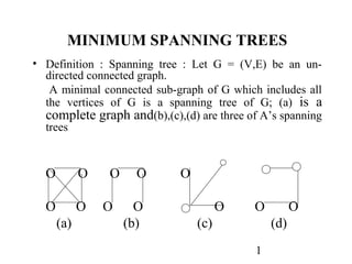
1. 1
MINIMUM SPANNING TREES
• Definition : Spanning tree : Let G = (V,E) be an un-
directed connected graph.
A minimal connected sub-graph of G which includes all
the vertices of G is a spanning tree of G; (a) is a
complete graph and(b),(c),(d) are three of A’s spanning
trees
O O O O O
O O O O O O O
(a) (b) (c) (d)

2. 2
APPLICATIONS OF SPANNING TREES
• Spanning trees can be used to obtain an
independent set of circuit equations for an
electrical network.
• Let B be the set of network edges not in the
spanning tree.
• Adding an edge from B to the spanning tree
creates a cycle.
• Different edges from B result in different cycles.

3. 3
APPLICATIONS OF SPANNING TREES
(Contd..)
• Kirchoff’s second law is used on each cycle
to obtain a circuit equation.
• The cycles obtained in this way are
independent as each contains one edge from
B which is not contained in any other cycle.
• Hence the circuit equations so obtained are
also independent.

4. 4
MINIMUM SPANNING TREES
• Thus a spanning tree is a minimal sub-graph G1
of
G such that V(G) = V(G1
) and G1
is connected.
• A connected graph with n vertices must have at
least n-1 edges and all connected graphs with n-1
edges are trees.
• If the nodes of G represent cities and the edges
represent possible communication links
connecting two cities, the minimum number of
links needed to connect the n cities is n-1.

5. 5
MINIMUM SPANNING TREES (Contd..)
• The spanning trees of G will represent all
feasible choices.
• In practice, the edges will have weights
associated with them.
• These might represent the cost of
construction, the length of the link etc.
• We are interested in finding a spanning
tree of G with minimum cost.

6. 6
Greedy method to obtain a minimum cost
spanning tree
Prim’s algorithm
• If A is the set of edges selected so far,
then A forms a tree.
• The next edges (u,v) to be included in A
is a minimum cost edge not in A with the
property that A U {u, v} is also a tree.

7. 7
Prim’s Algorithm for minimum cost spanning tree example
Example :Consider a graph G with 6 vertices as follows
2
10 50
1 40 3
45 35
5
30 25 15
55
4 6
20

8. 8
Prim’s Algorithm for minimum cost spanning tree
example (Contd..)
Edge Cost Spanning tree
(1,2) 10 10
1 2
(2,6) 25 10
1 2
6 25
(3,6) 15 10
1 2
25 6 15 3

9. 9
Prim’s Algorithm for minimum cost spanning tree
example (Contd..)
Edge Cost Spanning tree
(6,4) 20 10
1 2
25
4 20 6 15 3
(1,4) Reject
(3,5) 35 10
1 2 5
25
4 20 6 15 3 35
The cost of the spanning tree is 105

10. 10
PRIM’s algorithm to find minimum cost
spanning tree
Procedure PRIM (E,cost, n, T, mincost)
// E is the set of edges in G //
// cost (n,n) is the adjacency matrix //
// such as cost (i,j) is a +ve real number //
// or cost (i,j) is ∞ if no edge (i,j) exists //
// A minimum cost spanning tree is //
// computed and stored as a set //
// of edges in the array T(1:n-1, 2) //
// (T(i,1), T(i,2) is an edge in minimum cost spanning tree //

11. 11
PRIM’s algorithm to find minimum cost
spanning tree contd..
Real cost (n,n), mincost;
Integer near(n),i,j,k,l,T(1:n-1,2)
(k,l)  edge with minimum cost
4 mincost  cost (k,l)
(T(1,1) T(1,2) ) (k,l) // initialize spanning tree//
for i 1 to n do // with minimum cost edge
if cost (i, L) < cost (i, k) then // near(i) is one of
near (i)  L else near (i)  k // vertices of edges
endif // already included
repeat

12. 12
PRIM’s algorithm to find minimum cost
spanning tree contd..
10 near(k)  near (L)  0 // (k, L) is already
// in the tree or k and L are vertices in spanning tree
11 for i  2 to n-1 do //find n-2 additional
//edges for T //
12 Let j be an index such that
NEAR (J) ≠ 0 and COST (J,NEAR(J)) is
minimum

13. 13
PRIM’s algorithm to find minimum cost spanning tree contd..
(T(i,1),T(i,2))  (j, NEAR (j))
Mincost  mincost + cost (j, near (j))
NEAR (j)  0
16 for k  1 to n do // update near in view of newly
// included edge //
if NEAR (k) ≠ 0 and COST(k near (k)) > cost(k,j) then
NEAR (k)  j
endif
20 repeat // end for k is 1 to n
21 repeat // end for i is 2 to n-1
if mincost > ∞ then print (‘no spanning tree’)
endif
END PRIM
Complexity of Prim’s algorithm is O(n3
) ; n is the number of
vertices

14. 14
Explanation of Prim’s algorithm
• near(k) =0 means zero is a fictious vertex such that
cost(k,0) is always minimum; it means you need not find
any vertex near to K or L or near to any other vertex
already included in the spanning tree
• near (k) ≠ 0 means consider vertices which are not included
in the spanning tree
• After including a minimum cost edge near (i) is computed
for each i= 1,…n.
• Near (i) is the vertex (out of the two vertices in the
included edge) which is near to i.
• Near (i) is computed so that after including an edge, we
need to find the vertex with which we are trying to form the
new /next edge in the spanning tree.

15. 15
Explanation of Prim’s algorithm (Contd..)
• To exclude already included edges, make near (k) 0
near (L)  0 if (k, L) is included.
• In the second for-loop we are finding i which forms an
edge with near (i) and having minimum cost.
• In the third for-loop which is included in the second for-
loop we check whether near (i) values are same or, are to
be updated with respect to the newly added edge or w.r.t.
to the newly included vertex j.
• Updating near values is required because near(i) returns a
vertex (already in the spanning tree being formed) with
which edge is existing and to be included and it may
change dynamically due to inclusion of new edge and
hence new vertex
• For example near(3) is 2 and cost(3,2) is 50
when (2,6) is included, near(3) may be 1 or 2 or 6
As cost(3,6) < cost(3,2) (15 <50) near(3) is 6 (changed from 2 to 6)

16. 16
Explanation of Prim’s algorithm (Contd..)
Example:
Minimum cost edge (1, 2) with cost 10 is included
Near (3)  2
Near (4) 1
Near (5) 2
Near (6) 2
Near (1)  0
Near (2)0
Select out of 3,4,5,6 a vertex such that
{Cost (3, 2) = 50
Cost (4, 1) = 30
Cost (5, 2) = 40

17. 17
Explanation of Prim’s algorithm (Contd..)
Cost (6, 2) = 25} is minimum cleary it is 6 ∴j6
so the edge j, near (j) i.e. (6, 2) is included.
Now let us update near (k) values k =1…6
Near (1) = near (2) = near (6) = 0
K=3, cost (3, near (3) = 2) = 50 > cost (3, 6) =15
∴ near (3) is 6
near (4)  6  cost (4,1) = 30 > cost (4,6) = 20
near (5) 2  cost (5,2) = 40 < cost (5,6) = 55

18. 18
KRUSKAL’S ALGORITHM FOR
MINIMUM COST SPANNING TREE
• The edges are considered in the non
decreasing order.
• To get the minimum cost spanning tree, the
set of edges so far considered may not be a
tree; but with no cycles
• T will be a forest since the set of edges T
can be completed into a tree iff there are no
cycles in T.

19. 19
KRUSKAL’S ALGORITHM - Example
Example:
10
1 2
25 50
30 45 40 35 3
4 5
55 15
20 6

20. 20
KRUSKAL’S ALGORITHM – Example
(Contd..)
Edge Cost Spanning forest
(1,2) 10 1 2 3 4 5 6
(3,6) 15 1 2 3 4 5
6
(4,6) 20 1 2 3 5
4 6

21. 21
KRUSKAL’S ALGORITHM – Example
(Contd..)
Edge Cost Spanning forst
(2,6) 25 1 2 5
3
6
4
(1,4) 30 Reject ( T will form a cycle)
(3,5) 35 1 2 5
3
6
4
Stages in Kruskal’s algorithm.

22. 22
High level Kruskal’s algorithm
For minimum cost spanning tree
Let G = (V, E)
T  φ
While T contains fewer than (n-1)
edges and E ≠ φ do
• Choose an edge (v, w) from E of lowest cost.
• Delete (v, w) from E
• If (v, w) does not create a cycle in T,
then add (v, w) to T else discard (v, w).

23. 23
Implementation issues in Kruskal’s
algorithm for minimum cost spanning tree
• A tree with (n) vertices has (n-1) edges
• Minheap is used to delete minimum cost edge.
• To make sure that the added edge (v, w) does
not form a cycle in T, (to add to T), we use
UNION and FIND algorithms of sets.
• The vertices are grouped in such a way that all
the vertices in a connected component are placed
into a set
• Two vertices are connected in T iff they are in the
same set.

24. 24
Detailed Kruskal’s algorithm for minimum
cost spanning tree
Procedure Kruskal (E, cost, n, T, mincost)
// E is the set of edges in G. G has n vertices //
// cost (u, v) is the cost of edge (u , v)
T is the set of edges in the minimum cost spanning tree and mincost is
the cost //
real mincost, cost (1: n, 1:n)
integer parent (1: n), T(1:n-1, 2), n
Parent-1 //Each vertex is in a different set //
i mincost 0
While (i < n -1) and (heap not empty) do
delete a minimum cost edge (u,v) from the heap and reheapify using
ADJUST

25. 25
Detailed Kruskal’s algorithm for minimum
cost spanning tree contd..
JFIND (u); kFIND (v) // if j and k belong to the same set
If j ≠ k then ii+1 // they form a loop as already
T(i, 1)  u; T (i,2) v // existing edge can not be included
Mincost  mincost + cost(u,v)
Call union (j, k)
endif
Repeat if i ≠ n-1 // heap is empty but i ≠ n-1//
then “no spanning tree” endif
return
end KRUSKAL

26. 26
Detailed Kruskal’s algorithm for minimum
cost spanning tree- Example
Initially each vertex is in a different set {1}{2}{3}{4}{5}{6}
Consider(1, 2)
j1= Find(1); k = 2 = Find(2) 1 ≠2 so i1
(1,2) is included and union (1,2) = {1,2}
Consider (3,6) Test if (3,6) is forming a cycle with (1,2)
3 Find (3) 6 Find (6) 3 ≠ 6 so i2
(3,6) is included; UNION (3,6) = (3,6)
Consider (4,6); 4 Find(4) ; Find(6) is 3
3≠ 4 so i 3 and (4, 6) is added and union (3, 4) = (3, 4, 6)
Consider (2,6) Find(2) 1 [ union (1,3) is
Find(6) 3 union {1,2,3,4,6} ]

27. 27
Detailed Kruskal’s algorithm for minimum cost
spanning tree- Example contd..
Consider the next minimum cost edge (1, 4)
1 Find (1) 1 Find (4)
The root of the tree in which 1 and 4 belong
is the same; it means 1 and 4 form a cycle,
and hence (1,4) is rejected
Consider the next minimum cost edge (3, 5)
1 Find (3) 5 Find (5)
3 and 5 belong to different sets hence edge
(3,5) is included

28. 28
Complexity of Kruskal’s algorithm
• The edges are maintained as a min heap.
• The next edge can be obtained / deleted in
O(log e) time if G has e edges.
• Reconstruction of heap using ADJUST
takes O(e) time.
∴Kruskal’s algorithm takes O(e loge) time .

29. 29
Theorem: Kruskal’s algorithm generates a
minimum cost spanning tree
Proof: Let G be any undirected connected graph.
• Let T be the spanning tree for G generated by Kruskal’s
algorithm.
• Let T1
be a minimum cost spanning tree for G.
• We show that T and T1
have the same cost.
Let E(T) denote the set of edges in T
Let E(T1
) denote the set of edges in T1
• If n is the number of vertices in G, T and T’ have n-1
edges.
• If E(T) = E(T1
) then T is of minimum cost and theorem is
prooved.

30. 30
Proof of the theorem (contd..)
• Assume E(T) ≠ E(T1
).Then let e be a minimum cost edge.
• Such that e∈E(T) and e∉E(T1
) (not necessarily smallest
cost edge in E(T))
• Since T1
is a minimum cost spanning tree, the
inclusion of e in T1
creates a unique cycle.
• Let e, e1
, e2
, e3
…. ek
be this cycle.
• At least one of the ei
s 1≤ i ≤ k does not belong to
E(T); otherwise T will also contain this cycle.
• Let ej
is such that ej
∉E(T).
• We claim c(ej) ≥ c(e) (c( ) is the cost).

31. 31
Proof of the theorem (contd..)
• If c(ej
) < c(e) it would have been included into T.
• Also, all the edges in E(T) of cost less than the
cost of e are also in E(T1
) and do not form a cycle
with ej.
(e is an edge in E(T) and e∉E(T1
);
• Also E(T) and E(T1
) have the same number of
edges and hence they will have edges less cost
than e
• Now consider the graph with edge set E(T1
)U{e}.

32. 32
COMPLEXITY OF KRUSKAL’S
ALGORITHM (Contd..)
• Removal of any edge on the cycle e, e1
,e2
,….ek
will leave
behind a tree T11.
In particular, if we remove the edge ej
then
the resulting tree T11
will have a cost no more than the cost
of T1
.
• Hence T11
is also a minimum cost tree.
• By repeatedly using the transformation described
above, T1
can be transformed into the spanning
tree T without increase in cost.
• Hence T is a minimum cost spanning tree.

33. 33
SINGLE SOURCE SHORTEST
PATH PROBLEM
• Vertices in a graph may represent cities and edges may
represent sections of highway.
• The weights of edges may be distance between two cities
or the average time to drive from one city to the other.
The shortest path problem is as below :
• Given a directed graph = (V, E) a weighted function c(e)
for edges e of G and a source vertex V0
.
• The problem is to determine the shortest path from vo
to all
the remaining vertices of G.
• All weights are supposed to be positive.

34. 34
SINGLE SOURCE SHORTEST
PATH PROBLEM (Contd..)
Example:
45 Path Length
V0 50 V1 10 V4 1) V0V2 10
35 2) V0V2V3 25
10 20 20
30 3) V0V2V3V1 45
V2 V3 V5 4) V0V4 45
15 3
There is no path from V0 to V5

35. 35
GREEDY ALGORITHM TO
GENERATE SHORTEST PATH
• The paths are generated in non decreasing order of
path length. First a shortest path to the nearest
vertex is generated.
• Then a shortest path to the second nearest vertex is
generated and so on.
• We need to determine
• (i) the next vertex to which a shortest path must
be generated and
• (ii) a shortest path to this vertex.

36. 36
GREEDY ALGORITHM TO GENERATE
SHORTEST PATH (Contd..)
• Let S denote the set of vertices (including
vo
) to which the shortest paths have already
been generated.
• For w ∉ S, let Dist(w) be the length of the
shortest path starting from vo
going through
only those vertices which are in S and
ending at w.

37. 37
Observations in Greedy Algorithm
The following points need to be observed :
1. If the next shortest path is to vertex u, then the
path begins at vo ends at u and goes through only
those vertices which are in S.
• To prove this, assume there is a vertex w on this
path from Vo to u that is not in S. Thus the vo
to u
path also contains a path from vo to w which is of
length less than vo to u path.

38. 38
Observations in Greedy Algorithm
(Contd..)
By assumption the shortest paths are being
generated in non decreasing order of path length
and so the shortest path vo to w must already have
been generated.
Hence there can be no intermediate vertex which
is not in S.
(ii)The destination of the next path generated must
be the vertex which has the minimum distance
Dist (w) among all vertices not in S.

39. 39
Observations in Greedy Algorithm
(Contd..)
(iii)Having selected a vertex u as in (ii) and
generated the shortest vo to u path, vertex u
becomes a member of S.
- The value of Dist (w) may change.
- If it changes, the length of this path is
Dist (u) + c (u, w).

40. 40
DIJKSTRA’S SHORTEST PATH
ALGORITHM
Procedure SHORT-PATHS (v, cost, Dist, n)
// Dist (j) is the length of the shortest path from v to j in the
//graph G with n vertices; Dist (v) = 0 //
Boolean S(1:n); real cost (1:n,1:n), Dist (1:n); integer u, v, n,
num, i, w
// S(i) = 0 if i is not in S and s(i) =1 if it is in S//
// cost (i, j) = +α if edge (i, j) is not there//
// cost (i,j) = 0 if i = j; cost (i, j) = weight of < i, j > //
for i1 to n do // initialize S to empty //
S(i) 0; Dist (i) cost(v, i)
repeat

41. 41
DIJKSTRA’S SHORTEST PATH
ALGORITHM (Contd..)
// initially for no vertex shortest path is available//
S (v)1; dist(v)0// Put v in set S //
for num2 to n-1 do // determine n-1 paths from//
//vertex v //
choose u such that Dist (u)=min{dist(w)} and S(w)=0
S(u)1 // Put vertex u in S //
Dist(w)min (dist(w), Dist(u) + cost (u,w))
Repeat
repeat
end SHORT - PATHS

42. 42
Dijkstra’s shortest path algorithm
-example
Explanation of algorithm with example
45 S(1) = 0; S(2) = 0; …, S(5) = 0
Dist(1) cost (V0,V1) = 50
V0 50 V1 10 V4 Dist(2) cost (V0,V2)  10
15 Dist(3) cost (V0,V3) + α
35 Dist(4)  45; Dist(5)  α
20 10 20 Let S(V0) 1 Dist (V0)  0;
30 For num  2 to 4 do
V2 V3 V5 Dist(2) = min{Dist(1)…Dist(5)}
15 3 = 10
As vertex 2 is included, ∴U  2 ∴ S(2)  1

43. 43
Dijkstra’s shortest path algorithm –
example (Contd..)
Some of Dist(3), … Dist(5) may change
new Dist(3)  min (old Dist(3) = α, Dist(2)+cost(2,3))  min(α,10+15) = 25
new Dist(4)  min (old Dist(4) = 45, Dist(2)+cost(2,4))  min(45,10+α) = 45
new Dist(5)  min (old Dist(5) = α, Dist(2)+cost(2,5))  min(α,10+ α) = α
Now choose u such that dist (u)= min{Dist (3), Dist (4), Dist (5)))}
i.e min { 25, 45, α } = 25
∴U  3 S(3)  1
The process is continued.
The time taken by the algorithm is 0(n2
).

44. 44
Dijkstra’s shortest path algorithm –
example (Contd..)
• The edges on the shortest paths from a
vertex v to all remaining vertices in a
connected undirected graph G form a
spanning tree of G called shortest path
spanning tree.
• Shortest path spanning tree for the above
graph is :

45. 45
Dijkstra’s shortest path algorithm –
example (Contd..)
55 1 4 1
2 25 45 25 55 45
4 30 30 25
3 8 3 4 8 2 3 4 8
5 40 20 50 40 5 30
5 15 7 2 20 5 7
35 10 5 5 7 15
6 15 10
Graph G 10 6
6
minimum cost spanning tree G Shortest path spanning tree