v2

1. The Transition from Basal Crevasses to Rifts: The Role of Vertical Temperature Profile
Niall Coffey1, Ching-Yao Lai1,2, Yongji Wang2, W. Roger Buck3
1Program in Atmospheric and Oceanic Sciences, Princeton University
2Department of Geosciences, Princeton University
3Lamont-Doherty Earth Observatory, Columbia University
Summary
The Problem
Temperature Modification
Tensile Zero Toughness Crevasse Theories
1. For Nye’s Zero Stress, colder surface temperatures lower the
stress threshold for rift initiation. For Modified Nye’s Zero Stress,
temperature profile does not affect rift initiation stress. For
LEFM, colder surface temperatures increase the rift initiation
stress.
2. Yes, these theories re-predict rifts to occur where they have been
observed. Nye’s theory underpredicts rifts, particularly on
warmer ice shelves, whereas LEFM slightly overpredicts.
3. The range of rift initiation stress varies from 70% to 200% of the
freely floating stress,
4. Comparison of predictions with observed rifts shows most
agreement with a stress threshold just below or at the freely
floating stress. More observations of crevasses evolving into rifts
will help answer this question.
Comparison with Observations
Nye’s Zero Yield Stress (1955)
• A fracture will propagate until there is net compression at the crack tip.
• Assumes densely-spaced crevasses in incompressible, zero material strength ice where
flexural stresses cannot develop.
Motivation
The vertical fracture of
ice tongues and shelves
can lead to rifts and
iceberg calving, which
can reduce buttressing
stress and may increase
the rate of sea level rise.
1.How does a linear vertical temperature profile modify rift
initiation via basal crevasses across several theories?
2.Can these theories predict rifts to form via basal crevasses in
locations where rifts are observed?
3.What is the range of rift initiation stress predicted across
multiple theories given linear temperature profiles?
4.Do basal crevasses transition to rifts given stresses that are
buttressed, unbuttressed, or greater than unbuttressed?
Contact:
nbcoffey@princeton.edu
• Stress at the crack interface is
with resistive stress (Cuffey and Paterson, 2010)
• Temperature enters the resistive stress through ice hardness in our
effective rheology,
Modified Nye’s Zero Stress
• Ensure that horizontal force balance is upheld at the cracked location with dual surface
and basal crevasses. Adding temperature variation to simplified hardness yields the
system of equations with plotted solution on the right,
Nye’s Modified Nye’s LEFM
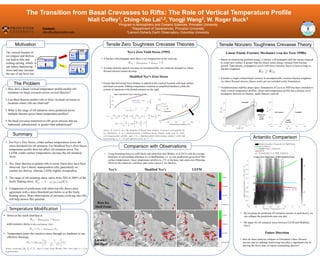
• Using bounding boxes to infill likely and identified rifts (Walker et al 2013) with the average
thickness of surrounding unbroken ice in BedMachine v2, we test predictions given RACMO
surface temperatures, linear temperature profiles to -2°C at the base, and strain rate (Wearing,
2016) on the relatively cold Ross and warm Larsen C Ice Shelves.
Antarctic Comparison
• By rescaling the predicted rift initiation stresses in each theory, we
can collapse the predictions onto one plot.
• We argue for rift initiation stress between LEFM and Modified
Nye’s.
Linear Elastic Fracture Mechanics (van der Veen 1998b)
• Based on minimizing potential energy, a fracture will propagate until the energy required
to create new surface is greater than the elastic strain energy released from fracture
growth. Equivalently, propagation occurs with stress intensity factor at least as large as
fracture toughness.
• Assumes a single isolated basal crevasse in incompressible, nonzero fracture toughness
ice where flexural stresses (future work) are not included in this formulation.
• Nondimensional stability phase space formulation of Lai et al 2020 has been extended to
study vertical temperature profiles, where each temperature profile has a distinct set of
boundaries between no fracture, stable fracture, and rift.
Unstable!
No Fracture Unstable!
Stable
Fracture
Future Direction
• How do these analyses compare in Greenland, where flexural
stresses and ice mélange buttressing may play a significant role in
altering the stress state of marine-terminating glaciers?
Repeat for
each T
profile
Ross Ice
Shelf Front
Larsen C
Ice Shelf
Tensile Nonzero Toughness Crevasse Theory

2. Hydrofracture Vulnerability in Greenland’s Ice Slab Areas
Riley Culberg, Yue Meng, Ching-Yao Lai
Department of Geosciences, Princeton University
Motivation Poromechanical Model
Application to the Greenland Ice Sheet
Will crevasses in ice slabs fill with water?
Are water-induced stresses sufficient to hydrofracture firn?
Non-Dimensional Analysis
Comparison of the rate of water infiltration into the
firn from the crevasse tip versus the rate at which
surface streams may feed water into a crevasse.
Blue bars show the plausible range of firn water
infiltration rates. Yellow bars show small stream
discharge values measured in the ablation zone of
Southwest Greenland. Red bars show large stream
discharges from the same region. Discharge from
the smallest streams is similar to the rate of leak-
off from the crevasse tip into the firn, so the
crevasse will not fill, preventing hydrofracture.
However, larger streams can inject water fast
enough to fill crevasses. Therefore, we also need to
understand whether the resulting water pressure in
the crevasse is sufficient to cause hydrofracture.
Firn Mechanical Properties
𝛿𝜎𝑥𝑥 𝑚𝑎𝑥
′
𝛽𝑏𝛿𝑝 −
𝜈
− 𝜈
𝜌𝑤𝑔 𝐻𝑤 − 𝐻𝑖
Constant Pressure
𝛿𝑝 𝜌𝑤𝑔𝐻𝑤
Constant Injection Velocity
𝛿𝑝
𝜋
𝜂𝑤𝑉𝑖𝑛𝑗𝐿𝑐𝑟𝑒𝑣
𝑘0
l
𝜂𝑤𝑉𝑖𝑛𝑗𝐿𝑐𝑟𝑒𝑣
𝜋𝜌𝑤𝑔𝑧0𝑘0
On the Greenland Ice Sheet, hydrofracture connects the supraglacial and subglacial
hydrologic systems, coupling surface runoff dynamics and ice velocity. Over the last two
decades, the growth of low-permeability ice slabs in the firn above the equilibrium line
has expanded Greenland’s runoff zone, but the vulnerability of these regions to
hydrofracture is still poorly understood. Observations from Northwest Greenland
suggest that when meltwater drains through crevasses in ice slabs, it is often stored in
the underlying relict firn layer and does not reach the ice sheet bed. However, there is
also evidence for the drainage of buried supraglacial lakes in this same region,
suggesting some eventual transition from infiltration to fracture.
Motivating Questions:
▪ What prevents water-filled crevasses in ice slabs from propagating unstably through
the underlying relict firn layer?
▪ What drives the observed transition to full ice thickness hydrofracture once all pore
space directly beneath a lake has been filled by refreezing?
Parameter Sweep
To apply the analytical model, we must define reasonable values for the physical, mechanical, and
hydraulic properties of ice slab-firn systems in Greenland. Unfortunately, given the sparse and
uncertain observations available, it is hard to choose a single representative value for any of these
parameters. Therefore, we take a Monte Carlo simulation approach. For each variable, we define
an empirical distribution of reasonable values using a compilation of in situ, laboratory, and remote
sensing measurements reported in the literature. For the hydraulic and mechanical properties, we
use various empirical relations to define these properties as a function of firn density.
Analytical model to calculate the maximum effective stress at the crack tip for ice slab-firn systems
and solid ice.
We use a two-phase poromechanics
model to simulate water injection into
a firn layer with constant pressure and
constant injection velocity boundary
conditions. We run a suite of
simulations with different mechanical
and hydraulic properties to develop an
analytical estimate of the maximum
effective stress in the firn.
Distributions of Effective Stress
Key Conclusions
• The firn layer beneath ice slabs imparts significant
resilience to hydrofracture because:
1) Leak-off into the firn may prevent crevasses from filling
with water
2) When crevasses do fill, much of the hydrostatic stress
is accommodated by a change in pore pressure, rather
than a being transmitted to the solid skeleton
• Surface-to-bed drainage connections are unlikely to form
until all local pore space has been filled with refrozen ice.
Non-dimensional maximum effective stress as a function of firn porosity and non-dimensional
water height in the crevasse. a) Water-filled crevasses. Effective stress increases with firn porosity
and water height due to the increasing water pressure, stronger fluid-solid coupling, and reduced
lithostatic stress. b) Supraglacial lake over a crevasse. Effective stress becomes more compressive
as the water level increases, due to the added lithostatic stress. As water level increases, firn
porosity plays a great role in determining the stress, since it modulates both the hydrostatic stress
transmitted to the solid skeleton, and the portion of the lithostatic stress transmitted horizontally.
Contact:
rtculberg@princeton.edu
Physically plausible distributions of maximum effective stress in firn (purple bars) and solid ice
(blue bars). a) Partially water-filled crevasse. The ice slab-firn and solid ice systems are similar, as
reduced overburden in the ice slab-firn system balances the complete transmission of hydrostatic
stress in the solid ice system. b) Mostly water-filled crevasse. Effective stress in the solid ice
system is tensile, but remains compressive in the ice slab-firn system, as pore pressure
accommodates much of the hydrostatic stress. c) Supraglacial lake overtop a crevasse. In the ice
slab-firn system, the effective stress becomes more compressive, because lithostatic stress
increases faster with lake depth than the portion of hydrostatic stress felt by the solid skeleton.
Biot Coefficient:
portion of stress felt by
the solid skeleton
Poisson’s Ratio:
portion of vertical stress
transmitted horizontally

3. Spontaneous Formation of Internal Shear Band of Ice Flowing Over A Complex Topography
Motivation
Emma Weijia Liu, Ludovic Räss, Frédéric Herman, Yury Podladchikov, Jenny Suckale
Department of Geophysics, Stanford University, Stanford, CA, USA liuwj@stanford.edu
As ice flows from ice divide to the ocean, it accelerates from less than 1 m/yr to
potentially more than 1 km/yr. The speed-up is thought to be associated with a
transition from flow through internal, distributed deformation to sliding,
accommodated by highly localized deformation at the ice-bedrock interface, often
referred to as flow-to-sliding transition. It remains unclear what mechanisms may
provide a viable explanation for the initiation and transition to sliding. We
investigate the impact of topographically uneven hard bedrock on ice flow
Thermo-mechanical Coupled Model
Hypothesis
Reference
Governing Equations
• Fluid equations :
!"!
!#!
= 0 ,
!$!"
!#"
−
!%
!#!
+ 𝑓& = 0
• Energy equation: 𝜌𝑐
!'
!(
+ 𝑢)
!'
!#!
=
!
!#!
𝜅
!'
!#!
+ 2𝜏)* ̇
𝜖)*
Bed topography and free surface
• Shear heating in the vicinity of pronounced roughness extends well into the
bulk of the ice, leading to a spatially variable viscosity and 3D flow field;
• Shear layer forms above the topography, leading to a potential internal highly
localized flow interface instead of rock-ice sliding interface.
Energy budget near the bed
Maier, Nathan, et al. "Sliding dominates slow-flowing margin regions, Greenland Ice Sheet." Science advances 5.7 (2019): eaaw5406.
Räss, Ludovic, et al. "Modelling thermomechanical ice deformation using a GPU-based implicit pseudo-transient method (FastICE v1. 0).“
Goldsby, D., & Kohlstedt, D. L. (2001). Superplastic deformation of ice: Experimental observations. Journal of Geophysical Research: Solid
Earth, 106 (B6),
Summary
• Ice flowing over a rough basal topography may spontaneously
develop an internal shear band on topographical highs.
• The shear strain rate localization and shear heating in the internal
shear band is amplified by a non-linear rheology.
• We identify two competing mechanisms that affect the energy
balance near the bedrock: vertical advective cooling and internal
shear heating.
About 50% of the internal deformation occurs within
the internal shear band
Define bandwidth of internal shear band
𝐵𝑤 = 𝑧 upper bound − 𝑧(lower bound)
𝐵𝑤∗ =
$!
%&
Formation of Internal Shear Band
How does the ice
start to slide?
Frozen bed Sliding bed
acceleration by
quantifying shear
localization in the vicinity
of the bedrock using
numerical simulations.
Rheology Models
The rheology governs the thermo-mechanical deformation of ice and hence the strain
localization that might occur within the ice column. In our model, we compare three
different constitutive relations, namely: a Newtonian rheology, a power law rheology,
and the composite rheology by Goldsby and Kohlstedt.
• Newtonian: Viscosity is a constant.
• Glen’s law:
̇
𝜖)* = 𝐴𝜏++
,-.
exp −
/
0 ''()*1'
• Composite:
̇
𝜖232 = ̇
𝜖4566 + ̇
𝜖7898: + ̇
𝜖;<=
-. + ̇
𝜖459:
We describe ice as an incompressible, non-linear, viscous fluid with
a temperature dependent rheology
• Immersed Boundary Methods: Fictitious domain method to
enforce no slip boundary condition at immersed bed.
𝐹
𝑖
𝑛+1/2
=
𝑈𝑑−𝑈𝑛
Δ𝑡
− 𝐺𝑛+
1
2, 𝑢𝑖
𝑛+1
= 𝑢𝑖
𝑛
+ 𝜏𝑢𝑖
𝑓𝑖
𝑛+1/2
• Level Set Methods: Represent the free surface as the level set
of a higher dimensional distance function, allowing us to
handle the moving front implicitly .
𝜕𝜙
𝜕𝑡
+ 𝑢𝑛 ∇𝜙 = 0
To identify how basal topography affects internal deformation, we compare the thermo-
mechanical deformation of ice flowing over an idealized sinusoidal topography to ice flowing
without topographical control.
We find that the shear
strain rate is highest
nearest to the bed,
whereas topography
shifts the shear-rate
maximum into the ice
column to a depth that is
corresponds roughly to
the height of the
topographic peaks. (a) and (b)shear strain rate shown in the background.
The velocity profiles at different locations along the
flow are shown in the dark green lines. (c) Shear
strain rate profile at x = 5000 m for both cases
To quantify the share of total deformation accommodated within the ice as ice flows over the
basal topography, we define the percentage of the internal deformation in the ice column to
be the ratio of the integral of the shear strain rate from the bed up to some elevation z and
the integral of the total shear strain rate in the entire ice column.
(a) Different wavelengths
(b) Different amplitudes
(a) and (b): The shear band development with and without a topography, defined
as a basal zone where the 50% of total deformation in the ice column occurs.
Here we use the lower and upper boundary of the shear band to be 20% and
70%. (c): The ratio of the shear band bandwidth to the ice thickness H at that
location along the flow for both cases
The bandwidth development along the flow for different topography
shapes. (a): Same amplitude of 100 m different wavelengths. (b): Same
wavelength of 263 m with different amplitudes.
We compare the rate of temperature change from only vertical advection (left
panels) to that of only shear heating (right panels) for the three rheology.
We find that non-linear rheology amplifies shear heating, thus overweighs
vertical cooling effect and results in positive energy balance near the bed .
Data source: (a) and (b): Background contour from BedMachine 3 (basal topography)
and MEaSUREs NSIDC (surface speed). (c): basal topography and surface speed
along flight line from Franke et al. (2021).
Scan for preprint
Geophysics Stanford

4. Improving Greenland Ice Sheet Freshwater Flux Parameterizations
Ellyn M. Enderlin1, Aman KC1, Dominik Fahrner2, Twila Moon3, Dustin Carroll4
1Boise State University, 2University of Oregon, 3National Snow and Ice Data Center, 4San Jose State University
Background
• Dynamic mass loss from marine-
terminating glaciers, called frontal or
terminus ablation, has two parts (Fig. 1):
(1) mass flux towards the terminus & (2)
mass removal from the terminus
• Terminus ablation is commonly estimated
as mass flux across a fixed inland “gate”
Ongoing Work
Revising terminus ablation estimates (Fig. 3)
• Focus on ~58 glaciers with good bed data near the terminus
• Flux across a fixed inland “gate” from Mankoff et al. (2020)
• Terminus delineations from TermPicks (Goliber et al., 2022)
• Filter spikes & dips in terminus change rate using near-
terminus flow speed from NASA ITS_LIVE
• Clip or extend delineations to fjord walls (Fig. 4)
• Terminus thickness from ArcticDEM & BedMachine bed
adjusted for surface elevation change using Khan (2017)
• Terminus ablation = discharge – terminus volume change
Estimating iceberg melt rates
1. Elevation-differencing method applied to all terminus
ablation sites: (method in Enderlin & Hamilton, 2014)
• manually map elevation changes using high-resolution
digital elevation models from 2011-present (Fig. 5)
• convert elevation change to meltwater fluxes using ice
density
• estimate melt rates orthogonal to a simplified
submerged geometry using meltwater flux, surface area,
and elevation data
2. Melt modeling with in situ ocean data:
• parameterize melt rates with in situ temperature +
salinity profiles & velocities from moorings near ~7
study sites
• Moon et al. (2018) iceberg melt model applied to a
range of iceberg geometries
Preliminary Results
• Basic code and dataset to be submitted for
review to Earth System Science Data (Fahrner et
al., in prep)
• (Fig. 6) Over decadal time scales, terminus
ablation is dominated by the “big 3”: Sermeq
Kujalleq (Jakobshavn), Helheim, & Kangerlussuaq
• Termpicks delineations resolve seasonal
variations in terminus position from ~2013-
present after filtering for changes that exceed
flow (mostly in automated delineation dataset)
• Seasonal terminus ablation pulses associated
with retreat (Fig. 7) can be orders of magnitude
greater than flux gate discharge
• Inter-annual variations in terminus ablation are
typically driven by discharge change, with much
small contributions from terminus
retreat/advance
Next Steps
• Augment terminus ablation pipeline to incorporate thickness changes from digital
elevation model timeseries
• Compare seasonal terminus ablation, mélange characteristic, & air and ocean
temperature reanalysis timeseries
• Expand elevation- and model-based iceberg melt datasets
References & Acknowledgements
This project is funded by NSF project “Improving estimates of Greenland’s freshwater flux: Where
do icebergs form and where do they melt?” (2052561/2052549/2052551) and the NSF-funded
Greenland Ice Sheet Ocean (GRISO) Science Network. Thank you to the GRISO Ocean Forcing Ice
Working Group for their help with the ESSD paper draft!
Mankoff et al. 2020 (doi:10.5194/essd-12-1367-2020); Goliber et al. 2022 (doi:10.5194/tc-16-3215-2022); Khan
2017 (http://promice.org/PromiceDataPortal/api/download/90fb4cbf-e88e-4e26-af95-a47d19a9cf10); Enderlin &
Hamilton 2014 (doi:10.3189/2014JoG14J085); Moon et al. 2018 (doi:10.1038/s41561-017-0018-z)
• Why iceberg production & decay matters:
• more precise knowledge of mass loss timing can
lead to insights on controls
• when & where ice is converted to liquid
freshwater may influence local-to-global ocean
circulation
• Our project’s goal is to develop Greenland
freshwater flux parameterizations that
account for variations in iceberg detachment
& melt in space and time (Fig. 2)
(top) Fig. 1:
Illustration of how
terminus ablation
can differ from
mass flux across
an inland gate for
several terminus
change scenarios.
(bottom) Fig. 2:
Project flowchart.
Objectives 1-2 are
described in the
ongoing work
section below.
Fig. 3: Flowchart outlining
terminus ablation
estimation process.
(above) Fig. 4: Modifications to terminus
delineations for mass change quantification.
(below) Fig. 5: Example of high-resolution
iceberg observations for melt estimation.
(above) Fig. 6: Cumulative terminus
ablation for 1987-2015. Symbols
colors denote magnitude and size
denotes percent for all sites.
(left) Fig. 7:
Terminus ablation
timeseries (a-c) and
terminus position
maps (d-f) for
Narsap Sermia,
Saqqarliup Sermia,
and Helheim
Gletsjer,
respectively.
Terminus
delineation colors
denote observation
year (see legend).
a) c)
b)
d) e) f)
Fig. 7b,e
Fig. 7a,d
Fig. 7c,f

5. Multiyear In Situ Proglacial Discharge from NW Greenland
Sarah E. Esenther1, Laurence C. Smith1, Adam Lewinter2, Lincoln H Pitcher3, Aaron Kehl2, Cuyler Onclin, Alexandra L. Boghosian4, Brandon Overstreet5, Seth Goldstein1
1Brown University Department of Earth, Environmental and Planetary Science, 2Cold Regions Research and Engineering Laboratory, 3Oak Ridge Institute for Science and
Education (ORISE), 4Lamont-Doherty Earth Observatory, 5Department of Geology and Geophysics, University of Wyoming
Background
Supraglacial runoff is the dominant pathway of ice mass loss
from the Greenland Ice Sheet (GrIS), but runoff projections
are poorly constrained in surface mass balance (SMB) models
of ice sheet loss. In many regions of the GrIS, in situ
measurement of discharge at proglacial stations for SMB
validation is complicated by the moulins and retentive firn.
We installed hydrometeorological stations at three grounded
watersheds in NW Greenland to capture daily, seasonal, and
interannual runoff patterns at high temporal (1 hour)
resolution, free of complication from en- and subglacial
interference.
Results
The first three years of observations (2019 to 2021) from these stations provide an ideal dataset for
comparison with RCM/SMB runoff. The long term dataset also provides insight into the seasonal
pattern of hydrology in NW Greenland: the meltwater runoff season lasts from ~late June to ~late
August/early September across the region; early onset of a strong diurnal runoff signal in 2019 and
2020 suggests minimal melt storage in snow or firn; the largest and sharpest floods in the region
appear to be triggered by late summer rain-on-ice events; statistical analysis indicates one-day
lagged air temperature, followed by ablation zone albedo, display the strongest correlation with
river flows and may drive interannual variations in hydrograph shape. AWS data are publicly
available through the PROMICE network (ING_1).
Instrumentation
The Minturn River cluster includes hydrological, meteorological, and time lapse camera
instrumentation, including a vented water level stage recorder and single shot lidar
accompanied by in situ terrestrial scanning lidar measurements. At the North River, single
shot lidar and pressure transducer instrumentation are supported by weather data from
the Thule Air Force Base airport weather station. Single shot lidar instrumentation was
installed at the Fox Canyon River in 2019 (a pressure transducer was added in 2022).
Figure 2. The first three years of hydrographs at the Minturn River. Seasonal and interannual
patterns were similar between the Minturn and North Rivers..
Figure 1. Gauging stations were installed at the surface-process
dominated Minturn (red), North (orange), and Fox Canyon (blue)
River watersheds. A weather station at the Minturn River (top)
transmits measurements hourly. Established and novel (e.g. single
beam lidar, left) instrumentation were installed to measure stage.
Fieldwork in 2019 and 2022 built stage-discharge curves at the
Minturn and North Rivers.
Funded by the NASA Cryospheric Science Program #80NSSC19K094

6. • Current fracture mechanics (i.e., LEFM) assumes that the stored elastic energy in an
impermeable solid matrix is instantaneously dissipated by creating new crack
surfaces, which only holds for impermeable solid media. Firn is porous material that
violates such assumption;
• We extend Biot’s poroelastic theory to two-phase immiscible flow to capture the
feedback between fluid flow and matrix deformation in the firn. We show that the
presence of a permeable firn layer prevents fracture propagation because a
significant portion of the hydrostatic stress is accommodated by changes in pore
pressure (~78% of total stress change), rather than being transmitted to the solid
skeleton (~22% of total stress change);
• To couple poromechanics, including thermoporoelasticity, thermoporoplasticity,
thermoporoviscoelasticity, with suitable glacial hydrology, rheology and fracture
models, to better understanding glacier dynamics.
Vulnerability of Firn to Hydrofracture: Poromechanics Modeling
Yue Meng, Riley Culberg, Ching-Yao Lai
Department of Geosciences, Princeton University
Motivation Poromechanics: The Concept of Effective Stress
Modeling Results Are water-induced stresses sufficient to hydrofracture firn?
Ice slabs are multi-meter thick layers of solid reforzen ice that form on top of the porous
firn layer in Greenland’s wet snow zone. Recent observations in Northwest Greenland
highlight the ability of this relict firn layer to store meltwater in its pores after surface
meltwater drains rapidly through cracks in the overlying ice slab. Current fracture
mechanics (i.e., LEFM) assumes that the stored elastic energy in an impermeable solid
matrix is instantaneously dissipated by creating new crack surfaces, which only holds for
impermeable solid media. To better understand the fate of meltwater in the porous firn
layer beneath ice slabs, we develop a two-dimensional, poroelastic continuum model to
quantify the stress and pressure changes in the porous firn during meltwater
penetration.
Motivating Questions:
▪ How does water infiltration affect the stresses in the porous firn layer, and how does
the maximum induced effective stress depend on the firn hydraulic or mechanical
properties (permeability, bulk modulus, porosity, etc)?
▪ How to apply poromechanics on the prediction of the hydrofracture vulnerability in
Greenland’s ice slab areas?
Analytical model to calculate the maximum effective stress at the crack tip for ice slab/firn systems and
solid ice. The poromechanical model predicts 𝛽 0.22.
When stress is applied to porous media, part of the stress is transmitted through the pore
fluid and part of the stress is transmitted through the solid skeleton. Effective stress—the
fraction of the total stress that is transmitted through the solid skeleton—controls the
mechanical behavior of porous media.
Contact:
om3193@princeton.edu
δ𝝈 𝛿𝝈′ − 𝑏𝛿𝑝𝑰
pore fluid (𝛿𝑝)
solid skeleton (𝛿𝜎′)
total stress (𝛿𝜎)
𝑏 −
𝐾
𝐾𝑠
∈ [0 ]
What is the fracture criterion for the porous firn?
0
0
2
Water injection into the firn induces a
tensile effective stress change at the
crevasse tip ( 𝛿𝜎𝑥𝑥
′ ). When the
horizontal effective stress exceeds the
firn tensile strength ( 𝜎𝑡
′
), vertical
fractures are generated. The fracture
criterion at the crevasse tip is written
as follows:
𝜎𝑥𝑥
′
𝜎𝑥𝑥 0
′
𝛿𝜎𝑥𝑥
′
≥ 𝜎𝑡
′
calculated from
lithostatic stress
calculated from
poromechanics
The 2D, Two-Phase Poroelastic Continuum Model
We use a 2D, two-phase poroelastic continuum model to solve the infiltration-induced stress
and pressure changes. The model has four governing equations, two derived from
conservation of fluid mass and two derived from conservation of linear momentum. The
model solves the time evolution of four unknowns: (1) pore pressure field 𝑝 𝑥 𝑧 𝑡 ; (2) water
saturation field 𝑆 𝑥 𝑧 𝑡 ; (3) horizontal displacement field 𝑢 𝑥 𝑧 𝑡 , and (4) vertical
displacement field 𝑤 𝑥 𝑧 𝑡 of the porous firn layer. The governing equations are summarized
and written in the x, z coordinates as follows:
Model set-up
𝟏. 𝜙
𝜕𝑆
𝜕𝑡
𝑆 𝑏
𝜕𝜖𝑘𝑘
𝜕𝑡 𝑀
𝜕𝑝
𝜕𝑡
−
𝑘0
𝜂𝑤
𝜕
𝜕𝑥
𝑘𝑟𝑤
𝜕𝑝
𝜕𝑥
−
𝑘0
𝜂𝑤
𝜕
𝜕𝑧
𝑘𝑟𝑤
𝜕𝑝
𝜕𝑧
− 𝜌𝑤𝑔 0;
𝟐. 𝑏
𝜕𝜖𝑘𝑘
𝜕𝑡 𝑀
𝜕𝑝
𝜕𝑡
− 𝑘0
𝜕
𝜕𝑥
𝑘𝑟𝑤
𝜂𝑤
𝑘𝑟𝑎
𝜂𝑎
𝜕𝑝
𝜕𝑥
−𝑘0
𝜕
𝜕𝑧
𝑘𝑟𝑤
𝜂𝑤
𝑘𝑟𝑎
𝜂𝑎
𝜕𝑝
𝜕𝑧
−
𝑘𝑟𝑤
𝜂𝑤
𝜌𝑤
𝑘𝑟𝑎
𝜂𝑎
𝜌𝑎 𝑔 0;
𝟑.
𝜕𝜎𝑥𝑥
𝜕𝑥
𝜕𝜎𝑧𝑥
𝜕𝑧
0;
𝟒.
𝜕𝜎𝑥𝑧
𝜕𝑥
𝜕𝜎𝑧𝑧
𝜕𝑧
− 𝜙 𝜌𝑠 𝜙 𝜌𝑎 − 𝑆 𝜌𝑤𝑆 𝑔 0.
δ𝝈 𝛿𝝈′ − 𝑏𝛿𝑝𝑰
𝛿𝝈′
𝛿𝝈′
3𝐾𝜈
𝜈
𝜖𝑘𝑘𝑰
3𝐾 − 2𝜈
𝜈
𝝐
Fluid continuity equations (for water and air phases):
Force balance equations (in x and z directions):
∗
𝑀
𝜙𝑆𝑐𝑤 𝜙 − 𝑆 𝑐𝑎 𝑏 − 𝜙 𝑐𝑠; 𝑘𝑟𝑤 𝑆3 𝑘𝑟𝑎 − 𝑆 2.
Here, we consider two scenarios of water infiltration into the porous firn layer:
▪ A constant water height (𝐻𝑤) in the surface crevasse;
▪ A constant water injection velocity (𝑉𝑖𝑛𝑗) at the crevasse tip.
How does the pore pressure or the skeleton stress
evolves during meltwater infiltration?
0
0.22
𝛿𝜎𝑥𝑥 𝑚𝑎𝑥
′
𝛽𝑏𝛿𝑝 −
𝜈
− 𝜈
𝜌𝑤𝑔 𝐻𝑤 − 𝐻𝑖
The poromechanical model predicts 𝛽 0.22.
Constant Pressure
𝛿𝑝 𝜌𝑤𝑔𝐻𝑤
Constant Injection Velocity
𝛿𝑝
2
𝜋
𝜂𝑤𝑉𝑖𝑛𝑗𝐿𝑐𝑟𝑒𝑣
𝑘0
l
2𝜂𝑤𝑉𝑖𝑛𝑗𝐿𝑐𝑟𝑒𝑣
𝜋𝜌𝑤𝑔𝑧0𝑘0
How does 𝜹𝝈𝒙𝒙 𝒎𝒂𝒙
′ depend on modeling parameters?
Analytical Expressions of 𝜹𝒑 and 𝜹𝝈𝒙𝒙 𝒎𝒂𝒙
′
Key Conclusions
Future Work
𝐻𝑖
porous firn
ice slab
𝑯𝒘
𝐻𝑖
impermeable solid ice
𝑯𝒘
Linear elastic fracture mechanics
(LEFM)
Poromechanics

7. Surprising surface similitude to bed topography in Greenland
1. Interpreting subglacial geology; and 2
1. Interpreting subglacial geology; and 2
1. Interpreting subglacial geology; and 2
Joseph A. MacGregor (joseph.a.macgregor@nasa.gov), Liam Colgan + GreenValley team
We’ve long known that prominent subglacial topographic features beneath the ice sheets can generate observable surface expressions. Recent advances in digital
elevation models (e.g., GrIMP) and bed-to-surface transfer theory now permit widespread observation of this phenomenon and easier interpretation. Hillshading a digital
elevation model across the direction of ice flow highlights major surface features nicely. For Greenland, comparison against NASA/KU/CReSIS airborne
radar-sounding data confirms that most features are due to subglacial topography and are typically valleys. This suggests a better path toward: 1. Interpolating subglacial
topography between sparse radar observations by developing methods that also require fidelity to observed surface relief; 2. Interpreting subglacial geology.
Bumps in the night
Sun valley slopes
GrIMP mosaic hillshaded
across the local direction
of ice flow (explained
below).
(A) Map of whole island
with manually traced
lineations overlain
(B–G) Zoom-ins of
selected regions with bed
elevation anomaly Δzb
(bed elevation minus 5-km
running mean) from
NASA/KU/CReSIS
radar-sounding tracks
overlain. Bed high / low.
(right column) Selected
radar-sounding tracks
from panels B–G with
along-track surface
elevation anomaly.
Ng et al. (2018)
How’d they do that?
1. Filter both the GrIMP DEM and MEaSUREs surface velocity using a 5H
thickness-dependent triangular filter and resample to a 5 km grid.
2. For the slower interior (< 100 m yr–1
), weight the flow direction toward filtered GrIMP
gradient direction.
3. Illuminate using a standard hillshade algorithm but allow illumination azimuth to vary for
each pixel, selecting the azimuth 90º counter-clockwise from the filtered ice-flow
direction. This direction consistently highlights coherent surface textures / lineations.
Next season
1. Invert for ice thickness and sliding rate across
the interior using a mono-layer model.
2. Better resolve subglacial geology using this
improved ice thickness and seismic, gravity
and magnetic data.
3. Hiring a new post-doc! Could be you!
v

8. Increasing extreme melt in northeast Greenland linked to foehn winds and atmospheric rivers
Kyle S. Mattingly 1
Jenny V. Turton 2
Jonathan D. Wille 3
Brice Noël 4
Xavier Fettweis 4
Åsa K. Rennermalm 5
Thomas L. Mote 6
1Space Science and Engineering Center (SSEC), University of Wisconsin-Madison 2Arctic Frontiers 3ETH Zurich 4University of Liège 5Rutgers, the State University of New Jersey 6University of Georgia
Introduction
Solid ice flow in northeast Greenland is dominated by the Northeast Greenland Ice Stream
(NEGIS), which drains ∼16% of the Greenland Ice Sheet. Its outlet glaciers contain over 1m
of potential sea level rise. NEGIS outlet glaciers have exhibited increasing mass loss in recent
years, due to warming air and ocean temperatures leading to the loss of buttressing sea ice and
ice shelf collapses at the floating glacier margins.
Ice flow dynamics in northeast Greenland are linked to surface hydrology. Glacier acceleration
can occur after surface melt events and supraglacial lake drainage. Extreme events can influence
firn structure across multiple melt seasons.
Previous studies have suggested a link between intense northeast Greenland melt events and
warm, dry downslope winds (”foehn”) descending from the ice sheet plateau to the west. Atmo‐
spheric rivers (ARs) affecting northwest Greenland may lead to foehn conditions and enhanced
melt in northeast Greenland after the moist air mass crosses the ice divide and flows downslope.
Figure 1. 20 July 2014 atmospheric river (AR) and melt event. (a) MERRA‐2 integrated water vapor transport (IVT),
500 hPa height, and AR outlines at 2014‐07‐20 1500 UTC. (b) RACMO2 simulated melt, 10‐m wind, and areas of
foehn conditions.
Research questions
1. What proportion of northeast Greenland summer melt is related to ARs in northwest
Greenland? How do AR contributions to extreme melt compare with all melt rates?
2. What role do foehn winds play in northeast Greenland melt? How are they related to
northwest Greenland ARs?
3. Have changes in the occurrence of ARs and foehn contributed to increasing northeast
Greenland melt?
Data and methods
AR detection algorithms (Mattingly and Wille) applied to MERRA‐2 data
Simulated summer (JJA) melt from RACMO2 model, validated using NASA MEaSUREs
Greenland Surface Melt Daily 25km EASE‐Grid 2.0 dataset
Foehn detection criteria applied to RACMO2:
Wind direction between 220◦
and 350◦
AND
Wind speed greater than 5 m s−1
AND
Relative humidity value <15th percentile of a two‐week window surrounding the given date OR
5% decrease in relative humidity AND 3◦
C increase in temperature compared to the previous six‐hour value
Northeast Greenland melt triggered by Western Greenland ARs
At higher elevations, 75–100% of summer surface melt is produced 0–48 hours after
northwest Greenland AR landfalls which occur with a seasonal frequency of 12–15% (13–16
days per summer).
At lower elevations, up to 75% of extreme (> 99th percentile) melt rates are associated with
northwest Greenland ARs.
Figure 2. Percentage of JJA surface melt attributable to ARs. Left column: the same day as AR landfall in western
Greenland; center column: 24 hours after AR landfall; right column: 48 hours after AR landfall. Top row is all melt
and bottom row is extreme (>99th percentile) melt.
Foehn winds drive most extreme melt events
In the lower NEGIS basin, 35–50% of melt occurs during the 25–40% of time when foehn
conditions occur.
Nearly all (75–100%) extreme (>99th percentile) melt in the lower NEGIS catchment occurs
with foehn conditions.
Figure 3. Influence of atmospheric rivers (ARs) and foehn conditions on northeast Greenland melt. (a)
Climatological mean JJA hourly melt in northeast Greenland. (b) Percentage of melt coincident with foehn
conditions during the 0–48 hour period after 90th percentile ARs (AR90) in northwest Greenland. (c) Temporal
evolution of foehn‐driven melt in northeast Greenland in 500m elevation bands during the ‐48 to +48 hour period
surrounding northwest Greenland ARs. (d) Percentage of extreme (>99th percentile) melt coincident with foehn.
Increasing strong ARs and extreme melt
Strong (AR90) events in northwest Greenland have increased during the 21st century.
AR90 events contribute disproportionately to melt in several recent years, especially when
paired with foehn conditions.
1980 1984 1988 1992 1996 2000 2004 2008 2012 2016
Year
0
2
4
6
AR
Frequency
(%)
r(pearson)=0.74
p-value=0.00
JJA (90th Percentile ARs)
Wille
Mattingly
Figure 4. AR90 trends in northwest Greenland from Wille Mattingly algorithms.
1980 1990 2000 2010 2020
0
20
40
60
80
No AR90, no foehn No AR90, foehn AR90, no foehn AR90, foehn
No AR90, no foehn No AR90, foehn AR90, no foehn AR90, foehn
%
of
JJA
melt
(solid);
%
of
time
(dashed)
Figure 5. Time series of northeast Greenland JJA melt attributable to combined AR and foehn conditions. Also
plotted is the percentage of time during which the given conditions occurred (dashed lines).
Outstanding questions
How will changes in regional sea ice affect foehn‐ and AR‐related melt in NE Greenland?
How will changes in large‐scale atmospheric circulation affect foehn‐ and AR‐related melt
in NE Greenland?
How do downsloping foehn winds affect melt in other regions of Greenland?
Paper reference
[Mattingly et al.(2023)Mattingly, Turton, Wille, Noël, Fettweis, Rennermalm, and Mote] Mattingly,
K. S., J. V. Turton, J. D. Wille, B. Noël, X. Fettweis, A. K. Rennermalm, and T. L. Mote,
Increasing extreme melt in northeast Greenland linked to foehn winds and atmospheric
rivers, Nature Communications, doi:10.1038/s41467-023-37434-8, 2023.
Acknowledgements
K. S. M. acknowledges support from the Polar Radiant Energy in the Far InfraRed Experiment (PRE‐
FIRE) mission, NASA grant 80NSSC18K1485. J. D. W. acknowledges support from the Agence
Nationale de la Recherche project, ANR‐20‐CE01‐0013 (ARCA). B. Noël was funded by the NWO
VENI grant VI.Veni.192.019.
Future Of Greenland ice Sheet Science (FOGSS) Workshop 2023 ksmattingly@wisc.edu

9. convolutional
Network Layers:
max pooling
fully connected
sigmoid
[m/yr]
Idealized ice sheet response to basal slipperiness
Josh Rines1, Ching-Yao Lai1,2, Yongji Wang2
(1) Program in Atmospheric and Oceanic Sciences, Princeton University
(2)Department of Geosciences, Princeton University
Motivation Reduced-Order Boundary Layer Model Empirical Scaling Relationships
Contact:
rinesjh@princeton.edu
Future/Ongoing Work
Rapid supraglacial lake drainages on the Greenland Ice Sheet (GrIS) margin are
thought to be often triggered by basal sliding in response to the presence of water at
the ice-bed interface. This sliding causes perturbations to the ice stress field which, if
strong enough, may overwhelm the ice fracture toughness leading to fracture formation
and/or propagation. It is therefore important to fundamentally understand the
relationship between sliding at the bed and the magnitude and lengthscale of the
induced stress response, specifically at the ice surface.
Motivating Questions:
§ What is the characteristic coupling lengthscale in response to basal slipperiness?
§ How does basal slipperiness control the lengthscale and magnitude of the ice surface
stress perturbation?
modified from Christoffersen et al., 2018
velocity field [m/yr], no slip case
velocity field [m/yr], free slip patch
∇ ⋅ 𝝈 + 𝒇! = 0
∇ ⋅ 𝒖 = 0
̇
𝜀 = 𝐴 𝑇 𝜏"($%)
; 𝑇 = −2℃
𝝈 ⋅ 2
𝒏 = 𝟎
ICE FLOW
ICE FLOW
𝝈 ⋅ 2
𝒏 = 𝟎
𝒖 = 𝟎
𝒖 = 𝟎
𝝉𝒃 = 𝟎
[m/yr]
[m/yr]
Stress perturbation magnitude & coupling length
stress magnitude
coupling length
surface stress [kPa], both cases
Along-flow 2D Stokes ice flow models (top) demonstrate the perturbation to the surface
stress (pink line in above) in response to a finite patch of basal slipperiness. From a
range of simulations with different ice surface profiles informed by continent-wide lake
locations [Dunmire et al., 2021], we observed an empirical relationship between ice
thickness and coupling length (bottom left), as well as between ice surface slope and
maximum perturbed stress (bottom right).
In order to more fundamentally understand the relationship between the
perturbations to the ice fields and the physical domain parameters (e.g., ice surface
slope, thickness, slip patch size), we constructed and analytically evaluated a
reduced-order boundary layer model. This model is sufficient to specify the scaling
relationship between the inner and outer solutions across the boundary layer at the
transition point between no-slip and free-slip.
Dimensionless outer problem (upstream):
on 𝑥 ∈ (0, 𝑥!)
at 𝑥 = 𝑥"
4𝜖(
ℎ 𝑢)
*
"
+*
𝑢) )
−
𝑢 ,+*
𝑢
ℎ
− ℎℎ) = 0
𝑢)
*
"
+*
𝑢) =
ℎ-
8𝜖(
Inner problem (boundary layer):
ℎ 𝑥 = 𝐻 𝑋 , 𝑢 𝑥 = 𝜖(.
𝑈 𝑋 , 𝑥- − 𝑥 = 𝜖(/
𝑋
at 𝑋 = 0
4𝜖
! "#$%
&%$
' 𝐻 𝑈(
"
'#"
𝑈( (
− 𝜖!&)
𝑈 )#"𝑈
𝐻
− 𝜖#!$
𝐻𝐻* = 0
𝜖
!
&#$
'
%"
𝑈(
"
'
#"
𝑈( =
𝐻+
8
on 𝑋 ∈ (∞, 0)
Extensional Shear Gravity pressure
Extensional and shear terms must balance
equation must balance
Rescale:
Constraint:
𝛼 = −
𝑛
𝑚 + 1
,
𝛽 =
𝑛𝑚
𝑚 + 1
Scalings:
ℎ 𝑥 = 𝐻 𝑋 ,
𝑢 𝑥 = 𝜖!"
#
$%&𝑈 𝑋 ,
𝑥' − 𝑥 = 𝜖"
#$
$%&𝑋
Newtonian rheology (n=m=1):
𝑥'
∗ − 𝑥∗
[𝑥]
= 𝜖𝑋 ⇒ 𝑥'
∗ − 𝑥∗ = 𝑧 𝑋
𝜖 =
[𝑧]
[𝑥]
Boundary layer extent scales linearly
with ice thickness (H)
[m/yr]
Boundary layer is linear with
thickness (𝒖𝑩𝑳 = 𝒖𝒍𝒆𝒇𝒕 ∗ 𝒖𝒓𝒊𝒈𝒉𝒕 )
Repeated the simulation for different ice thicknesses and patch sizes to investigate the
scaling between patch size and boundary layer extent, for example a 10 km patch:
Simulations
Simulations
Continent-wide
lake locations
Continent-wide
lake locations
𝒛
𝒙
Boundary layer extent scales
linearly with ice thickness (H)
Derived a rescaled relationship for
boundary layer extent (L) as a
function of thickness (H) and patch
size (l)
Boundary layer extent defined as Rxx
convergence to background (noslip)
state
The analytical scaling and the
results from the simulations
provide good evidence that for a
Newtonian rheology the
boundary layer extent, or in other
words the coupling length, scales
linearly with ice thickness, both
throughout the thickness of the
ice as well as between
simulations of different
thicknesses. The exact boundary
layer extent additionally depends
on ice viscosity and slippery
patch length (l).
We repeated the above
simulation for different ice
thicknesses but a common
surface slope and computed the
boundary layer extent for each
simulation as the convergence of
the surface to the background
level defined by a no-slip basal
boundary condition reference
case. This boundary layer can be
thought of as the extent
upstream from the slippery patch
that the basal perturbation is felt
at the surface.
Boundary layer project:
• Solve inner problem explicitly
• Utilize physics-informed neural network (PINN) to obtain analytical solution
• Match the inner and outer solutions to obtain an overall solution
• Obtain a scaling relationship between surface slope and stress magnitude
• Extend analytical analysis to a Glen flow law rheology
• Extend analysis numerically to more realistic boundary conditions and viscoelastic rheologies
GrIS surface feature identification project:
• Create a CNN workflow to accurately identify fracture density in the GrIS ablation zone
• Extend CNN workflow to identify moulins in the GrIS ablation zone
Input imagery:
Fracture density
[0,1]
(294x294x4)
(147x147x8)
(73x73x8) (36x36x8)
(1x1x10368) (1x1x1)
WorldView tiles
𝐿 ∝ 𝐻𝑙!
, 𝛼 ≈ 0.1

10. 38% of Greenland’s Marine Terminating
Glaciers (MTG) are Non-Categorized
(relative to fjord/ice geometry and
Atlantic Water presence) but this
knowledge gap is responsible for nearly
20% of recent GrIS ice loss and 15% of
annual discharge (1992-2017)
therefore GO-MARIE launched in 2022
to map those gaps.
Note: Whereas MTG is n=226 glacier associated with
Wood et al. 2021
The Ocean Research Project (ORP), a
US-based NGO mobilizes for the
international hydrographic mapping
needs around the GrIS through the
decadal campaign, GO-MARIE
(Glacier-Ocean Mapping & Research
Interdisciplinary Effort)
ORP contributed hydrographic data to
NASA OMG in 2015-16, and 2018.
GO-MARIE Observations Include:
• glacial fjord bathymetry
During Peak GrIS melt period:
• ocean temperature
• current velocity
• Suspended sediment
concentration
Intended to support ….
• Categorizing fjord/ice geometry
• Identifying the Presence/Absence
of Atlantic Water
Observations are made:
< 1km from a
Marine Terminating Glacier defined as
1. non-categorized (Wood, 2021) 2. or
associated with a poor bathymetry
fjord (Choi, 2021). 3. underestimated
or underinvestigaited sites like West
Greenland’s .
Wood, Michael & Rignot, E. & Fenty, Ian & An, Lu & Bjørk, Anders & Van den Broeke,
Michiel & Cai, Cilan & Kane, Emily & Menemenlis, Dimitris & Millan, Romain &
Morlighem, Mathieu & Mouginot, Jeremie & Noël, Brice & Scheuchl, Bernd &
Velicogna, Isabella & Willis, Josh & Zhang, Hong. (2021). Ocean forcing drives glacier
retreat in Greenland. Science Advances. 7. eaba7282. 10.1126/sciadv.aba7282.
Choi, Y., Morlighem, M., Rignot, E. et al. Ice dynamics will remain a primary driver of
Greenland ice sheet mass loss over the next century. Commun Earth Environ 2, 26
(2021). https://doi.org/10.1038/s43247-021-00092-z
Catania, Ginny & Stearns, L. & Sutherland, D. & Fried, Mason & Bartholomaus, Timothy
& Morlighem, Mathieu & Shroyer, E. & Nash, J.. (2018). Geometric Controls on
Tidewater Glacier Retreat in Central Western Greenland. Journal of Geophysical
Research: Earth Surface. 123. 10.1029/2017JF004499.
Version 2.0: Moon, T., Fisher, M., Harden, L., Simonoko, H., and T. Stafford
(2022). QGreenland (v2.0.0) [software], National Snow and Ice Data Center.
GO-MARIE Addresses GrIS Glacial Fjord
Hydrographic Mapping Needs 2022-2030
trenholm.orp@gmail.com www.oceanresearchproject@gmail.com
Planned
Mapped
(2022)
NW
NW
W
S
E
SRV Marie Tharp moves from pole mounted multibeam sonar (2022) to hull mounted
in 2023. 22m and crew compliment up to 9 including a 4 science party of 4.
Partners
Instruments
Archives
GO-MARIE Requires:
• Survey & Observation
Type Review at FOGSS
• Survey Funding
• Securing deeper ranging
acoustics: > 400-600 m
sonar and > 70 m ranging
ADCP
• Committed Collabs
• Strategy for an inclusive &
decolonized campaign
Near Bed Topography
Multibeam Survey Plan 2022+
Catania et al. 2018
Landsat
Nicole Trenholm
trenholm.orp@gmail.com
References
Models
NCEI DCDB IBCAO – GEBCO - BedMachine
• Workhorse Sentinel ADCP 600 khz (70 m range)
• Reson 7125 (200-400 khz) to 500m
• RBR CTD with multiple sensors
2022:
Glacial Fjord
Multibeam
Surveys: 400 km2,
100+ CTDs, ADCP,
Physical sampling:
cores, water,
sediment
Dedicated campaigns for improved
GrIS modeling during the Ocean Decade
Ice Velocity
and landmass
from
QGreenland

11. Bias correction and statistical modeling of variable oceanic forcing of Greenland outlet glaciers
Vincent Verjans1, Alexander Robel1, Andy Thompson2, and Hélène Seroussi3
1 Georgia Institute of Technology, 2 California Institute of Technology, 3 Dartmouth College
vverjans3@gatech.edu
Introduction
- Variability in oceanic conditions directly impacts ice loss from
marine outlet glaciers in Greenland.
- Oceanic conditions are available from Atmosphere-Ocean Global
Climate Model (AOGCM) output, but these models require extensive
computational resources and lack the fine resolution needed to
simulate ocean dynamics on the Greenland continental shelf and
close to glacier marine termini (𝒪(100m-1km) vs. 𝒪(100km)).
- We develop a statistical approach to generate ocean forcing for ice
sheet models, incorporating spatio-temporal variability and trends.
𝑇𝐹 (thermal forcing)
is defined as the
temperature above
local melting point
integrated between
0-500 m depth. 𝑇𝐹
shown is from (c).
Overview
1) Correct mean and
variability of
AOGCMs using
ocean reanalyses.
(Quantile Delta
Mapping)
2) Extrapolate
offshore TF to
inshore, based on
constraints from
high-resolution
(𝒪(1km)) ocean
model.
3) Calibrate statistical
time series
emulator to spatio-
temporal patterns.
We generate stochastic ensembles of time series
reproducing spatio-temporal variability of ocean
conditions at negligible computational expense.
Methods
1) Quantile Delta Mapping (QDM)
- Calibrates the Cumulative Density Function (CDF) of the AOGCM 𝑇𝐹 to the
CDF of the reanalysis 𝑇𝐹 → captures mean and variability amplitude
- For future projections, modeled relative changes are preserved.
- Allows to combine fidelity with respect to reanalysis and modeled trends and
temporal patterns.
2) Offshore-to-Inshore extrapolation
- Use constraints from output of the high-resolution ECCO2-Arctic runc
(4km).
- Separate 𝑇𝐹 time series in components: mean (𝑇𝐹), trend ( ሶ
𝑇𝐹), seasonality (𝑇𝐹𝑆), residuals (𝑇𝐹′).
- Derive offshore-to-inshore regression relations for each TF component from the ECCO2-Arcic TF spatial patterns.
- Find the optimal offshore AOGCM grid point predictor for any given glacier (see Box).
- Apply the regression relations to the QDM-corrected AOGCM TF time series of the selected offshore predictor grid point.
3) Statistical time series models
- Capturing temporal characteristics of inshore QDM-corrected time series,
- Reproducing spatial correlations between Greenland glaciers.
- Accounting for internal climate variability via a stochastic parameterization.
- Computationally efficient.
- Mean, trend, and seasonality are represented with piecewise polynomials.
- Residual variability is modeled as an Autoregressive Moving-Average
(ARMA) process → statistics of residual variability are calibrated to the
QDM-corrected inshore AOGCM values.
Box: Finding the optimal offshore AOGCM grid point predictor
Across all the AOGCM grid points, we minimize a cost function accounting for:
- agreement between ECCO2-Arctic and the QDM-corrected AOGCM
- agreement between offshore and inshore ECCO2-Arctic
- offshore-to-inshore distance
Each 𝑇𝐹 component has its own cost function:
Example of QDM: AOGCM time series calibrated to reanalysis.
Example of extrapolation procedure for the three 𝑇𝐹, 𝑇𝐹𝑆, and 𝑇𝐹 components.
Example of a deterministic QDM-corrected and extrapolated 𝑇𝐹, and
statistical realizations. σ: standard deviation, ρ1: 1-year autocorrelation
Example of a sparse
correlation matrix for
𝑇𝐹 at the 226
Greenland glaciers of
out dataset.
Example of cost
functions computed
for 𝑇𝐹 components
at Helheim glacier.
Conclusions
- Our method is complimentary, and can further improve, current 𝑻𝑭 parameterizations for Greenland.
- 𝑻𝑭 distribution correction, extrapolation, and statistical model fitting are independent and can be performed individually.
- Our method is agnostic to the choice of (1) reanalysis productd, (2) high-resolution ocean modelc, (3) AOGCMe,f.
- This procedure is well-suited for generating large ensembles of 𝑻𝑭 realizations to force ice sheet model simulations.
- Four already-processed ensembles of 1000 𝑻𝑭 time series (1850-2100) each, and all the source code are openly availableb.
a, Verjans et al.,: Bias correction and statistical modeling of variable oceanic forcing of Greenland outlet glaciers. doi: 10.22541/essoar.167397462.24826991/v1, 2023, in review. b, Dataset associated (Verjans et al., 2023): https://doi.org/10.5281/zenodo.7478350
c, Nguyen et al.: Source and pathway of the western arctic upper halocline in a data-constrained coupled ocean and sea ice model. doi: 10.1175/JPO-D-11-040.1, 2012. d, Good et al.: EN4: Quality controlled ocean temperature and salinity profiles and monthly objective analyses with uncertainty estimates. doi: 0.1002/2013JC009067, 2013
e, Hajima et al.: Development of the MIROC-ES2L Earth System Model and the evaluation of biogeochemical processes and feedbacks. doi: 10.5194/gmd-13-2197-2020, 2020. f, Boucher et al.: Presentation and evaluation of the IPSL-CM6A-LR climate model. doi: 10.1029/2019MS002010, 2020.
𝑇𝐹: long-term mean, 𝑇𝐹𝑆: seasonality
𝑇𝐹′
: residual variability, ሶ
𝑇𝐹: long-term trend
cr: coarse-resolution AOGCM,
hr: high-resolution ocean model
in: inshore, off: offshore
𝑀𝑖: monthly effect at month 𝑖, σ: standard deviation
δ(𝑡, 𝑖): delta function time step 𝑡 in month 𝑖