Signal & systems

Signal
• A signal is a pattern of variation that carry information.
• Signals are represented mathematically as a function of
one or more independent variable
• A picture is brightness as a function of two spatial
variables, x and y.
• In this course signals involving a single independent
variable, generally refer to as a time, t are considered.
Although it may not represent time in specific application
• A signal is a real-valued or scalar-valued function of an
independent variable t.

Signal Examples
• Electrical signals --- voltages and currents in a circuit
• Acoustic signals --- audio or speech signals (analog
or digital)
• Video signals --- intensity variations in an image (e.g.
a CAT scan)
• Biological signals --- sequence of bases in a gene
• Noise: unwanted signal
:

Measuring Signals
-1
-0.8
-0.6
-0.4
-0.2
0
0.2
0.4
0.6
0.8
1
1 22 43 64 85 106 127 148 169 190 211 232 253 274 295 316 337 358 379 400 421 442 463 484 505 526 547 568 589 610 631 652 673 694 715
Period
Amplitude

Definitions
• Voltage – the force which moves an electrical current
against resistance
• Waveform – the shape of the signal (previous slide is a
sine wave) derived from its amplitude and frequency
over a fixed time (other waveform is the square wave)
• Amplitude – the maximum value of a signal, measured
from its average state
• Frequency (pitch) – the number of cycles produced in a
second – Hertz (Hz). Relate this to the speed of a
processor eg 1.4GigaHertz or 1.4 billion cycles per
second

Signal Basics
 Continuous time (CT) and discrete time (DT) signals
CT signals take on real or complex values as a function of an independent
variable that ranges over the real numbers and are denoted as x(t).
DT signals take on real or complex values as a function of an independent
variable that ranges over the integers and are denoted as x[n].
Note the subtle use of parentheses and square brackets to distinguish between
CT and DT signals.

Analog Signals
• Human Voice – best example
• Ear recognises sounds 20KHz or less
• AM Radio – 535KHz to 1605KHz
• FM Radio – 88MHz to 108MHz

Digital signals
• Represented by Square Wave
• All data represented by binary values
• Single Binary Digit – Bit
• Transmission of contiguous group of bits is a bit
stream
• Not all decimal values can be represented by
binary
1 0 1 0 1 0 1 0

Analogue vs. Digital
Analogue Advantages
• Best suited for audio and video
• Consume less bandwidth
• Available world wide
• Less susceptible to noise
Digital Advantages
• Best for computer data
• Can be easily compressed
• Can be encrypted
• Equipment is more common and less expensive
• Can provide better clarity

Analog or Digital
• Analog Message: continuous in amplitude and over
time
– AM, FM for voice sound
– Traditional TV for analog video
– First generation cellular phone (analog mode)
– Record player
• Digital message: 0 or 1, or discrete value
– VCD, DVD
– 2G/3G cellular phone
– Data on your disk
– Your grade
• Digital age: why digital communication will prevail

A/D and D/A
• Analog to Digital conversion; Digital to
Analog conversion
– Gateway from the communication device to the
channel
• Nyquist Sampling theorem
– From time domain: If the highest frequency in the
signal is B Hz, the signal can be reconstructed
from its samples, taken at a rate not less than 2B
samples per second

A/D and D/A
• Quantization
– From amplitude domain
– N bit quantization, L intervals L=2N
– Usually 8 to 16 bits
– Error Performance: Signal to noise ratio

Real vs. Complex
Q. Why do we deal with complex signals?
A. They are often analytically simpler to deal with than real
signals, especially in digital communications.

What is a communications
system?
• Communications Systems: Systems
designed to transmit and receive
information
Info
Source
Info
Source
Info
Sink
Info
Sink
Comm
System

Block Diagram
Receiver
Rx
received
message
to
sink
)(~ tm
Transmitter
Tx s(t)
transmitted
signal
Channel
r(t)
received
signal
m(t)
message
from
source
Info
Source
Info
Source
Info
Sink
Info
Sink
n(t)
noise

A discrete-time signal is defined at discrete
times.

Elementary Signals
Sinusoidal & Exponential Signals
• Sinusoids and exponentials are important in signal and
system analysis because they arise naturally in the
solutions of the differential equations.
• Sinusoidal Signals can expressed in either of two ways :
cyclic frequency form- A sin 2Пfot = A sin(2П/To)t
radian frequency form- A sin ωot
ωo= 2Пfo= 2П/To
To= Time Period of the Sinusoidal Wave

Sinusoidal & Exponential Signals Contd.
x(t) = A sin (2Пfot+ θ)
= A sin (ωot+ θ)
x(t) = Aeat Real Exponential
= Aejω̥t =
A[cos (ωot) +j sin (ωot)] ComplexExponential
θ = Phase of sinusoidal wave
A = amplitude of a sinusoidal or exponential signal
fo= fundamental cyclic frequency of sinusoidal signal
ωo= radian frequency
Sinusoidal signal

Unit Step Function
( )
1 , 0
u 1/ 2 , 0
0 , 0
t
t t
t
>

= =
 <
Precise Graph Commonly-Used Graph

Signum Function
( ) ( )
1 , 0
sgn 0 , 0 2u 1
1 , 0
t
t t t
t
> 
 
= = = − 
 − < 
Precise Graph Commonly-Used Graph
The signum function, is closely related to the unit-step
function.

Unit Ramp Function
( ) ( ) ( )
, 0
ramp u u
0 , 0
t
t t
t d t t
t
λ λ
−∞
> 
= = = 
≤ 
∫
•The unit ramp function is the integral of the unit step function.
•It is called the unit ramp function because for positive t, its
slope is one amplitude unit per time.

Rectangular Pulse or Gate Function
Rectangular pulse, ( )
1/ , / 2
0 , / 2
a
a t a
t
t a
δ
 <
= 
>

Unit Impulse Function
( )
( )
As approaches zero, g approaches a unit
step andg approaches a unit impulse
a t
t′
So unit impulse function is the derivative of the unit step
function or unit step is the integral of the unit impulse
function
Functions that approach unit step and unit impulse

Representation of Impulse Function
The area under an impulse is called its strength or weight. It is
represented graphically by a vertical arrow. An impulse with a
strength of one is called a unit impulse.

Properties of the Impulse Function
( ) ( ) ( )0 0g gt t t dt tδ
∞
−∞
− =∫
The Sampling Property
( )( ) ( )0 0
1
a t t t t
a
δ δ− = −
The Scaling Property
The Replication Property
g(t)⊗ δ(t) = g (t)

Unit Impulse Train
The unit impulse train is a sum of infinitely uniformly-
spaced impulses and is given by
( ) ( ) , an integerT
n
t t nT nδ δ
∞
=−∞
= −∑

The Unit Rectangle Function
The unit rectangle or gate signal can be represented as combination
of two shifted unit step signals as shown

The Unit Triangle Function
A triangular pulse whose height and area are both one but its base
width is not, is called unit triangle function. The unit triangle is
related to the unit rectangle through an operation called
convolution.

Sinc Function
( )
( )sin
sinc
t
t
t
π
π
=

Discrete-Time Signals
• Sampling is the acquisition of the values of a
continuous-time signal at discrete points in time
• x(t) is a continuous-time signal, x[n] is a discrete-
time signal
[ ] ( )x x where is the time between sampless sn nT T=

Discrete Time Exponential and
Sinusoidal Signals
• DT signals can be defined in a manner analogous to their
continuous-time counter part
x[n] = A sin (2Пn/No+θ)
= A sin (2ПFon+ θ)
x[n] = an
n = the discrete time
A = amplitude
θ = phase shifting radians,
No = Discrete Period of the wave
1/N0= Fo= Ωo/2 П = Discrete Frequency
Discrete Time Sinusoidal Signal
Discrete Time Exponential Signal

Discrete Time Sinusoidal Signals

Discrete Time Unit Step Function or
Unit Sequence Function
[ ]
1 , 0
u
0 , 0
n
n
n
≥
= 
<

Discrete Time Unit Ramp Function
[ ] [ ]
, 0
ramp u 1
0 , 0
n
m
n n
n m
n =−∞
≥ 
= = − 
< 
∑

Discrete Time Unit Impulse Function or
Unit Pulse Sequence
[ ]
1 , 0
0 , 0
n
n
n
δ
=
= 
≠
[ ] [ ] for any non-zero, finite integer .n an aδ δ=

Unit Pulse Sequence Contd.
• The discrete-time unit impulse is a function in the
ordinary sense in contrast with the continuous-
time unit impulse.
• It has a sampling property.
• It has no scaling property i.e.
δ[n]= δ[an] for any non-zero finite integer ‘a’

Operations of Signals
• Sometime a given mathematical function may
completely describe a signal .
• Different operations are required for different
purposes of arbitrary signals.
• The operations on signals can be
Time Shifting
Time Scaling
Time Inversion or Time Folding

Time Shifting
• The original signal x(t) is shifted by an
amount tₒ.
• X(t)X(t-to) Signal Delayed Shift to the
right

Time Shifting Contd.
• X(t)X(t+to) Signal Advanced Shift
to the left

Time Scaling
• For the given function x(t), x(at) is the time
scaled version of x(t)
• For a 1,period of function x(t) reduces and˃
function speeds up. Graph of the function
shrinks.
• For a 1, the period of the x(t) increases˂
and the function slows down. Graph of the
function expands.

Time scaling Contd.
Example: Given x(t) and we are to find y(t) = x(2t).
The period of x(t) is 2 and the period of y(t) is 1,

Time scaling Contd.
• Given y(t),
– find w(t) = y(3t)
and v(t) = y(t/3).

Time Reversal
• Time reversal is also called time folding
• In Time reversal signal is reversed with
respect to time i.e.
y(t) = x(-t) is obtained for the given
function

0 0, an integern n n n→ +Time shifting
Operations of Discrete Time
Functions

Operations of Discrete Functions Contd.
Scaling; Signal Compression
n Kn→ K an integer > 1

Classification of Signals
• Deterministic & Non Deterministic Signals
• Periodic & A periodic Signals
• Even & Odd Signals
• Energy & Power Signals

Deterministic & Non Deterministic Signals
Deterministic signals
• Behavior of these signals is predictable w.r.t time
• There is no uncertainty with respect to its value at any
time.
• These signals can be expressed mathematically.
For example x(t) = sin(3t) is deterministic signal.

Deterministic & Non Deterministic Signals
Contd.
Non Deterministic or Random signals
• Behavior of these signals is random i.e. not predictable
w.r.t time.
• There is an uncertainty with respect to its value at any
time.
• These signals can’t be expressed mathematically.
• For example Thermal Noise generated is non
deterministic signal.

Periodic and Non-periodic Signals
• Given x(t) is a continuous-time signal
• x (t) is periodic iff x(t) = x(t+Tₒ) for any T and any integer n
• Example
– x(t) = A cos(ωt)
– x(t+Tₒ) = A cos[ω(t+Tₒ)] = A cos(ωt+ωTₒ)= A cos(ωt+2π)
= A cos(ωt)
– Note: Tₒ =1/fₒ ; ω=2πfₒ

Periodic and Non-periodic Signals
Contd.
• For non-periodic signals
x(t) ≠ x(t+Tₒ)
• A non-periodic signal is assumed to have a
period T = ∞
• Example of non periodic signal is an
exponential signal

Important Condition of Periodicity for
Discrete Time Signals
• A discrete time signal is periodic if
x(n) = x(n+N)
• For satisfying the above condition the
frequency of the discrete time signal should
be ratio of two integers
i.e. fₒ = k/N

Sum of periodic Signals
• X(t) = x1(t) + X2(t)
• X(t+T) = x1(t+m1T1) + X2(t+m2T2)
• m1T1=m2T2 = Tₒ = Fundamental period
• Example: cos(tπ/3)+sin(tπ/4)
– T1=(2π)/(π/3)=6; T2 =(2π)/(π/4)=8;
– T1/T2=6/8 = ¾ = (rational number) = m2/m1
– m1T1=m2T2  Find m1 and m2
– 6.4 = 3.8 = 24 = Tₒ

Sum of periodic Signals – may not
always be periodic!
T1=(2π)/(1)= 2π; T2 =(2π)/(sqrt(2));
T1/T2= sqrt(2);
– Note: T1/T2 = sqrt(2) is an irrational number
– X(t) is aperiodic
tttxtxtx 2sincos)()()( 21 +=+=

Even and Odd Signals
Even Functions Odd Functions
gt()=g−t() gt()=−g−t()

Even and Odd Parts of Functions
( )
( ) ( )g g
The of a function is g
2
e
t t
t
+ −
=even part
( )
( ) ( )g g
The of a function is g
2
o
t t
t
− −
=odd part
A function whose even part is zero, is odd and a function
whose odd part is zero, is even.

Various Combinations of even and odd
functions
Function type Sum Difference Product Quotient
Both even Even Even Even Even
Both odd Odd Odd Even Even
Even and odd Neither Neither Odd Odd

Product of Two Even Functions
Product of Even and Odd Functions

Product of Even and Odd Functions Contd.
Product of an Even Function and an Odd Function

Product of an Even Function and an Odd Function

Product of Two Odd Functions

Derivatives and Integrals of Functions
Function type Derivative Integral
Even Odd Odd + constant
Odd Even Even

Discrete Time Even and Odd Signals
[ ]
[ ] [ ]g g
g
2
e
n n
n
+ −
= [ ]
[ ] [ ]g g
g
2
o
n n
n
− −
=
[ ] [ ]g gn n= − [ ] [ ]g gn n= − −

Combination of even and odd
function for DT Signals
Function type Sum Difference Product Quotient
Both even Even Even Even Even
Both odd Odd Odd Even Even
Even and odd Even or Odd Even or odd Odd Odd

Products of DT Even and Odd
Functions
Two Even Functions

Functions Contd.
An Even Function and an Odd Function

Proof Examples
• Prove that product of two even
signals is even.
• Prove that product of two odd
signals is odd.
• What is the product of an even
signal and an odd signal? Prove
it!
)()()(
)()()(
)()()(
21
21
21
txtxtx
txtxtx
txtxtx
=×
=−×−=−
→×=
Eventx
txtxtx
txtxtx
txtxtx
←−
=−=−×
=−×−=−
→×=
)(
)()()(
)()()(
)()()(
21
21
21
Change t -t

Functions Contd.
Two Odd Functions

Energy and Power Signals
Energy Signal
• A signal with finite energy and zero power is called
Energy Signal i.e.for energy signal
0<E<∞ and P =0
• Signal energy of a signal is defined as the area
under the square of the magnitude of the signal.
• The units of signal energy depends on the unit of the
signal.
( )
2
x xE t dt
∞
−∞
= ∫

Energy and Power Signals Contd.
Power Signal
• Some signals have infinite signal energy. In that
caseit is more convenient to deal with average
signal power.
• For power signals
0<P<∞ and E = ∞
• Average power of the signal is given by
( )
/ 2
2
x
/ 2
1
lim x
T
T
T
P t dt
T→∞
−
= ∫

Energy and Power Signals Contd.
• For a periodic signal x(t) the average signal
power is
• T is any period of the signal.
• Periodic signals are generally power signals.
( )
2
x
1
x
T
P t dt
T
= ∫

Signal Energy and Power for DT
Signal
•The signal energy of a for a discrete time signal x[n] is
[ ]
2
x x
n
E n
∞
=−∞
= ∑
•A discrtet time signal with finite energy and zero
power is called Energy Signal i.e.for energy signal
0<E<∞ and P =0

Signal Energy and Power for DT
Signal Contd.
The average signal power of a discrete time power signal
x[n] is
[ ]
1
2
x
1
lim x
2
N
N
n N
P n
N
−
→∞
=−
= ∑
[ ]
2
x
1
x
n N
P n
N =
= ∑
For a periodic signal x[n] the average signal power is
The notation means the sum over any set of
consecutive 's exactly in length.
n N
n N
=
 
 ÷
 ÷
 
∑

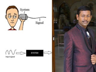
What is System?
• Systems process input signals to produce output
signals
• A system is combination of elements that
manipulates one or more signals to accomplish a
function and produces some output.
system output
signal
input
signal

Examples of Systems
– A circuit involving a capacitor can be viewed as a
system that transforms the source voltage (signal) to the
voltage (signal) across the capacitor
– A communication system is generally composed of three
sub-systems, the transmitter, the channel and the
receiver. The channel typically attenuates and adds
noise to the transmitted signal which must be processed
by the receiver
– Biomedical system resulting in biomedical signal
processing
– Control systems

System - Example
• Consider an RL series circuit
– Using a first order equation:
dt
tdi
LRtitVVtV
dt
tdi
LtV
LR
L
)(
)()()(
)(
)(
+⋅=+=
=
LV(t)
R

Mathematical Modeling of Continuous
Systems
Most continuous time systems represent how continuous
signals are transformed via differential equations.
E.g. RC circuit
System indicating car velocity
)(
1
)(
1)(
tv
RC
tv
RCdt
tdv
sc
c
=+
)()(
)(
tftv
dt
tdv
m =+ ρ

Mathematical Modeling of Discrete
Time Systems
Most discrete time systems represent how discrete signals are
transformed via difference equations
e.g. bank account, discrete car velocity system
][]1[01.1][ nxnyny +−=
][]1[][ nf
m
nv
m
m
nv
∆+
∆
=−
∆+
−
ρρ

Order of System
• Order of the Continuous System is the highest
power of the derivative associated with the output
in the differential equation
• For example the order of the system shown is 1.
)()(
)(
tftv
dt
tdv
m =+ ρ

Order of System Contd.
• Order of the Discrete Time system is the
highest number in the difference equation
by which the output is delayed
• For example the order of the system shown
is 1.
][]1[01.1][ nxnyny +−=

Interconnected Systems
notes
• Parallel
• Serial (cascaded)
• Feedback
LV(t)
R
L
C

Interconnected System Example
• Consider the following systems with 4 subsystem
• Each subsystem transforms it input signal
• The result will be:
– y3(t)=y1(t)+y2(t)=T1[x(t)]+T2[x(t)]
– y4(t)=T3[y3(t)]= T3(T1[x(t)]+T2[x(t)])
– y(t)= y4(t)* y5(t)= T3(T1[x(t)]+T2[x(t)])* T4[x(t)]

Feedback System
• Used in automatic control
– e(t)=x(t)-y3(t)= x(t)-T3[y(t)]=
– y(t)= T2[m(t)]=T2(T1[e(t)])
  y(t)=T2(T1[x(t)-y3(t)])= T2(T1( [x(t)] - T3[y(t)] ) ) =
– =T2(T1([x(t)] –T3[y(t)]))

Types of Systems
• Causal & Anticausal
• Linear & Non Linear
• Time Variant &Time-invariant
• Stable & Unstable
• Static & Dynamic
• Invertible & Inverse Systems

Causal & Anticausal Systems
• Causal system : A system is said to be causal if
the present value of the output signal depends only
on the present and/or past values of the input
signal.
• Example: y[n]=x[n]+1/2x[n-1]

Causal & Anticausal Systems Contd.
• Anticausal system : A system is said to be
anticausal if the present value of the output
signal depends only on the future values of
the input signal.
• Example: y[n]=x[n+1]+1/2x[n-1]

Linear & Non Linear Systems
• A system is said to be linear if it satisfies the
principle of superposition
• For checking the linearity of the given system,
firstly we check the response due to linear
combination of inputs
• Then we combine the two outputs linearly in the
same manner as the inputs are combined and again
total response is checked
• If response in step 2 and 3 are the same,the system
is linear othewise it is non linear.

Time Invariant and Time Variant
Systems
• A system is said to be time invariant if a time
delay or time advance of the input signal leads to a
identical time shift in the output signal.
0
0 0
( ) { ( )}
{ { ( )}} { ( )}
i
t t
y t H x t t
H S x t HS x t
= −
= =
0
0
0 0
( ) { ( )}
{ { ( )}} { ( )}
t
t t
y t S y t
S H x t S H x t
=
= =

Stable & Unstable Systems
• A system is said to be bounded-input bounded-
output stable (BIBO stable) iff every bounded
input results in a bounded output.
i.e.
| ( ) | | ( ) |x yt x t M t y t M∀ ≤ < ∞ → ∀ ≤ < ∞

Stable & Unstable Systems Contd.
Example
- y[n]=1/3(x[n]+x[n-1]+x[n-2])
1
[ ] [ ] [ 1] [ 2]
3
1
(| [ ]| | [ 1]| | [ 2]|)
3
1
( )
3
x x x x
y n x n x n x n
x n x n x n
M M M M
= + − + −
≤ + − + −
≤ + + =

Stable & Unstable Systems Contd.
Example: The system represented by
y(t) = A x(t) is unstable ; A 1˃
Reason: let us assume x(t) = u(t), then at
every instant u(t) will keep on multiplying
with A and hence it will not be bonded.

Static & Dynamic Systems
• A static system is memoryless system
• It has no storage devices
• its output signal depends on present values of the
input signal
• For example

Static & Dynamic Systems Contd.
• A dynamic system possesses memory
• It has the storage devices
• A system is said to possess memory if its output
signal depends on past values and future values of
the input signal

Example: Static or Dynamic?
Answer:
• The system shown above is RC circuit
• R is memoryless
• C is memory device as it stores charge
because of which voltage across it can’t
change immediately
• Hence given system is dynamic or memory
system

Invertible & Inverse Systems
• If a system is invertible it has an Inverse System
• Example: y(t)=2x(t)
– System is invertible must have inverse, that is:
– For any x(t) we get a distinct output y(t)
– Thus, the system must have an Inverse
• x(t)=1/2 y(t)=z(t)
y(t)
System
Inverse
System
x(t) x(t)
y(t)=2x(t)System
(multiplier)
Inverse
System
(divider)
x(t) x(t)

LTI Systems
• LTI Systems are completely characterized by its
unit sample response
• The output of any LTI System is a convolution of
the input signal with the unit-impulse response,
i.e.

Properties of Convolution
Commutative Property
][*][][*][ nxnhnhnx =
Distributive Property
])[*][(])[*][(
])[][(*][
21
21
nhnxnhnx
nhnhnx
+
=+
Associative Property
][*])[*][(
][*])[*][(
][*][*][
12
21
21
nhnhnx
nhnhnx
nhnhnx
=
=

Useful Properties of (DT) LTI Systems
• Causality:
• Stability:
Bounded Input ↔ Bounded Output
00][ <= nnh
∞<∑
∞
−∞=k
kh ][
∞<−≤−=
∞<≤
∑∑
∞
−∞=
∞
−∞= kk
knhxknhkxny
xnx
][][][][
][for
max
max

Signal & systems

Recomendados

Recomendados

Más contenido relacionado

La actualidad más candente

La actualidad más candente (20)

Similar a Signal & systems

Similar a Signal & systems (20)

Más de AJAL A J

Más de AJAL A J (20)

Último

Último (20)

Signal & systems

Notas del editor