1 ECONOMICS 581: LECTURE NOTES CHAPTER 4: MICROECONOMIC THEORY: A DUAL APPROACH W. Erwin Diewert March 2011. 1. Introduction In this chapter, we will show how the theory of convex sets and concave and convex functions can be useful in deriving some theorems in microeconomics. Section 2 starts off by developing the properties of cost functions. It is shown that without assuming any regularity properties on an underlying production function, the corresponding function satisfies a large number of regularity properties. Section 3 shows how the cost function can be used to determine a production function that is consistent with a given cost function satisfying the appropriate regularity conditions. Section 4 establishes the derivative property of the cost function: it is shown that the first order partial derivatives of the cost function generate the firm’s system of cost minimizing input demand functions. Section 5 shows how the material in the previous sections can be used to derive the comparative statics properties of the producer’s system of cost minimizing input demand functions. Section 6 asks under what conditions can we assume that the technology exhibits constant returns to scale. Section 7 indicates that price elasticities of demand will tend to decrease in magnitude as a production model becomes more aggregated. Section 8 notes that the duality between cost and production functions is isomorphic or identical to the duality between utility and expenditure functions. In this extension of the previous theory, the output level of the producer is replaced with the utility level of the consumer, the production function of the producer is replaced with the utility function of the consumer and the producer’s cost minimization problem is replaced by the problem of the consumer minimizing the expenditure required to attain a target utility level. Thus the results in the first 5 sections have an immediate application to the consumer’s system of Hicksian demand functions. The final sections of the chapter return to producer theory but it is no longer assumed that only one output is produced; we extend the earlier analysis to the case of multiple output and multiple input technologies. 2. Properties of Cost Functions The production function and the corresponding cost function play a central role in many economic applications. In this section, we will show that under certain conditions, the cost function is a sufficient statistic for the corresponding production function; i.e., if we know the cost function of a producer, then this cost function can be used to generate the underlying production function. 2 Let the producer’s production function f(x) denote the maximum amount of output that can be produced in a given time period, given that the producer has access to the nonnegative vector ...

1. 1
ECONOMICS 581: LECTURE NOTES
CHAPTER 4: MICROECONOMIC THEORY: A DUAL
APPROACH
W. Erwin Diewert
March 2011.
1. Introduction
In this chapter, we will show how the theory of convex sets and
concave and convex
functions can be useful in deriving some theorems in
microeconomics. Section 2 starts
off by developing the properties of cost functions. It is shown
that without assuming any
regularity properties on an underlying production function, the
corresponding function
satisfies a large number of regularity properties. Section 3
shows how the cost function
can be used to determine a production function that is consistent
with a given cost
function satisfying the appropriate regularity conditions.
Section 4 establishes the
derivative property of the cost function: it is shown that the
first order partial derivatives
of the cost function generate the firm’s system of cost
minimizing input demand
functions. Section 5 shows how the material in the previous
sections can be used to

2. derive the comparative statics properties of the producer’s
system of cost minimizing
input demand functions. Section 6 asks under what conditions
can we assume that the
technology exhibits constant returns to scale. Section 7
indicates that price elasticities of
demand will tend to decrease in magnitude as a production
model becomes more
aggregated.
Section 8 notes that the duality between cost and production
functions is isomorphic or
identical to the duality between utility and expenditure
functions. In this extension of the
previous theory, the output level of the producer is replaced
with the utility level of the
consumer, the production function of the producer is replaced
with the utility function of
the consumer and the producer’s cost minimization problem is
replaced by the problem
of the consumer minimizing the expenditure required to attain a
target utility level. Thus
the results in the first 5 sections have an immediate application
to the consumer’s system
of Hicksian demand functions.
The final sections of the chapter return to producer theory but it
is no longer assumed that
only one output is produced; we extend the earlier analysis to
the case of multiple output
and multiple input technologies.
2. Properties of Cost Functions
The production function and the corresponding cost function
play a central role in many

3. economic applications. In this section, we will show that under
certain conditions, the
cost function is a sufficient statistic for the corresponding
production function; i.e., if we
know the cost function of a producer, then this cost function can
be used to generate the
underlying production function.
2
Let the producer’s production function f(x) denote the maximum
amount of output that
can be produced in a given time period, given that the producer
has access to the
nonnegative vector of inputs, x ≡ [x1,…,xN] ≥ 0N. If the
production function satisfies
certain regularity conditions,1 then given any positive output
level y that the technology
can produce and any strictly positive vector of input prices p ≡
[p1,…,pN] >> 0N, we can
calculate the producer’s cost function C(y,p) as the solution
value to the following
constrained minimization problem:
(1) C(y,p) ≡ minx {pTx : f(x) ≥ y ; x ≥ 0N}.
It turns out that the cost function C will satisfy the following 7
properties, irrespective of
the properties of the production function f.
Theorem 1; Diewert (1982; 537-543)2: Suppose f is continuous
from above. Then C
defined by (1) has the following properties:

4. Property 1: C(y,p) is a nonnegative function.
Property 2: C(y,p) is positively linearly homogeneous in p for
each fixed y; i.e.,
(2) C(y,λp) = λC(y,p) for all λ > 0, p >> 0N and y∈ Range f
(i.e., y is an output level that
is producible by the production function f).
Property 3: C(y,p) is nondecreasing in p for each fixed
y∈ Range f; i.e.,
(3) y∈ Range f, 0N << p1 < p2 implies C(y,p1) ≤ C(y,p2).
Property 4: C(y,p) is a concave function of p for each fixed
y∈ Range f; i.e.,
(4) y∈ Range f, p1 >> 0N; p2 >> 0N; 0 < λ < 1 implies
C(y,λp1+(1−λ)p2) ≥ λC(y,p1) + (1−λ)C(y,p2).
Property 5: C(y,p) is a continuous function of p for each fixed
y∈ Range f.
Property 6: C(y,p) is nondecreasing in y for fixed p; i.e.,
(5) p >> 0N, y1∈ Range f, y2∈ Range f, y1 < y2 implies C(y1,p)
≤ C(y2,p).
Property 7: For every p >> 0N, C(y,p) is continuous from below
in y; i.e.,
(6) y*∈ Range f , yn∈ Range f for n = 1,2,…, yn ≤ yn+1,
limn→∝y
n = y* implies
limn→∝ C(y

5. n,p) = C(y*,p).
1 We require that f be continuous from above for the minimum
to the cost minimization problem to exist;
i.e., for every output level y that can be produced by the
technology (so that y∈ Range f), we require that the
set of x’s that can produce at least output level y (this is the
upper level set L(y) ≡ {x : f(x) ≥ y}) is a closed
set in RN.
2 For the history of closely related results, see Diewert (1974a;
116-120).
3
Proof of Property 1: Let y∈ Range f and p >> 0N. Then
C(y,p) ≡ minx {pTx : f(x) ≥ y ; x ≥ 0N}
= pTx* where x* ≥ 0N
and f(x*) ≥ y
≥ 0 since p >> 0N
and x* ≥ 0N.
Proof of Property 2: Let y∈ Range f, p >> 0N and λ > 0. Then
C(y,λp) ≡ minx {λpTx : f(x) ≥ y ; x ≥ 0N}
= λ minx {pTx : f(x) ≥ y ; x ≥ 0N} since λ > 0
= λC(y,p) using the
definition of C(y,p).
Proof of Property 3: Let y∈ Range f, 0N << p1 < p2. Then
C(y,p2) ≡ minx {p2Tx : f(x) ≥ y ; x ≥ 0N}

6. = p2Tx* where f(x*) ≥ y
and x* ≥ 0N
≥ p1Tx* since x* ≥ 0N
and p2 > p1
≥ minx {p1Tx : f(x) ≥ y ; x ≥ 0N} since x* is
feasible for this problem
≡ C(y,p1).
Proof of Property 4: Let y∈ Range f, p1 >> 0N; p2 >> 0N; 0 < λ
< 1. Then
C(y,λp1+(1−λ)p2) ≡ minx {[λp1+(1−λ)p2]Tx : f(x) ≥ y ; x ≥
0N}
= [λp1 + (1−λ)p2]Tx* where x* ≥ 0N
and f(x*) ≥ y
= λp1Tx* + (1−λ)p2Tx*
≥ λ minx {p1Tx : f(x) ≥ y ; x ≥ 0N} +
(1−λ)p2Tx*
since x* is feasible for the cost
minimization problem that uses
the price vector p1 and using also λ >
0
= λC(y,p1) + (1−λ)p2Tx* using the
definition of C(y,p1)
≥ λC(y,p1) + (1−λ) minx {p2Tx : f(x) ≥ y ;
x ≥ 0N}
since x* is feasible for the cost
minimization problem that uses
the price vector p2 and using also
1−λ > 0
= λC(y,p1) + (1−λ)C(y,p2) using the
definition of C(y,p2).
Figure 1 below illustrates why this concavity property holds.

7. 4
In Figure 1, the isocost line {x: p1Tx = C(y,p1)} is tangent to
the production possibilities
set L(y) ≡ {x: f(x) ≥ y, x ≥ 0N} at the point x1 and the isocost
line {x: p2Tx = C(y,p2)} is
tangent to the production possibilities set L(y) at the point x2.
Note that the point x**
belongs to both of these isocost lines. Thus x** will belong to
any weighted average of
the two isocost lines. The λ and 1−λ weighted average isocost
line is the set {x:
[λp1+(1−λ)p2]Tx = λC(y,p1) + (1−λ)C(y,p2)} and this set is the
dotted line through x** in
Figure 1. Note that this dotted line lies below3 the parallel
dotted line that is just tangent
to L(y), which is the isocost line {x: [λp1+(1−λ)p2]Tx =
[λp1+(1−λ)p2]Tx* =
C(y,λp1+(1−λ)p2)} and it is this fact that gives us the concavity
inequality (4).
Proof of Property 5: Since C(y,p) is a concave function of p
defined over the open set of
p’s, Ω ≡ {p: p >> 0N}, it follows that C(y,p) is also continuous
in p over this domain of
definition set for each fixed y∈ Range f.4
Proof of Property 6: Let p >> 0N, y1∈ Range f, y2∈ Range f, y1
< y2. Then
C(y2,p) ≡ minx {pTx : f(x) ≥ y2 ; x ≥ 0N}
≥ minx {pTx : f(x) ≥ y1 ; x ≥ 0N}

8. since if y1 < y2, the set {x : f(x) ≥ y2} is a subset
of the set {x : f(x) ≥ y1} and
the minimum of a linear function over a bigger set
cannot increase
≡ C(y1,p).
Proof of Property 7: The proof is rather technical and may be
found in Diewert (1993;
113-114).
Q.E.D.
3 It can happen that the two dotted lines coincide.
4 See Fenchel (1953; 75) or Rockafellar (1970; 82).
Figure 1: The Concavity in Prices Property of the Cost Function
x2
x1
x1
x2
x*
C(y,p1)/p21
C(y,p2)/p22
C(y,pλ)/p2λ
[λC(y,p1) +
(1−λ)C(y,p2)]/p2λ
L(y)

9. Output level y isoquant or
indifference curve in the consumer
context
x**
5
Problems
1. In industrial organization,5 it used to be fairly common to
assume that a firm’s cost
function had the following linear functional form: C(y,p) ≡ α +
βTp + γy where α and γ
are scalar parameters and β is a vector of parameters to be
estimated econometrically.
What are sufficient conditions on these N+2 parameters for this
cost function to satisfy
properties 1 to 7 above? Is the resulting cost function very
realistic?
2. Suppose a producer’s production function, f(x), defined for
x∈ S where S ≡ {x: x ≥ 0N}
satisfies the following conditions:
(i) f is continuous over S;
(ii) f(x) > 0 if x >> 0N and
(iii) f is positively linearly homogeneous over S; i.e., for every
x ≥ 0N and λ > 0, f(λx) =
λf(x).
Define the producer’s unit cost function c(p) for p >> 0N as
follows:
(iv) c(p) ≡ C(1,p) ≡ minx {pTx : f(x) ≥ 1 ; x ≥ 0N};
i.e., c(p) is the minimum cost of producing one unit of output if

10. the producer faces the
positive input price vector p. For y > 0 and p >> 0N, show that
(v) C(y,p) = c(p)y.
Note: A production function f that satisfies property (iii) is
said to exhibit constant
returns to scale. The interpretation of (v) is that if a production
function exhibits
constant returns to scale, then total cost is equal to unit cost
times the output level.
3. Shephard (1953; 4) defined a production function F to be
homothetic if it could be
written as
(i) F(x) = g[f(x)] ; x ≥ 0N
where f satisfies conditions (i)-(iii) in Problem 2 above and
g(z), defined for all z ≥ 0,
satisfies the following regularity conditions:
(ii) g(z) is positive if z > 0;
(iii) g is a continuous function of one variable and
(iv) g is monotonically increasing; i.e., if 0 ≤ z1 < z2, then
g(z1) < g(z2).
Let C(y,p) be the cost function that corresponds to F(x). Show
that under the above
assumptions, for y > 0 and p >> 0N, we have
(v) C(y,p) = g−1(y)c(p)
where c(p) is the unit cost function that corresponds to the
linearly homogeneous f and
g−1 is the inverse function for g; i.e., g−1[g(z)] = z for all z ≥
0. Note that g−1(y) is a
monotonically increasing continuous function of one variable.
3. The Determination of the Production Function from the Cost
Function
The material in the previous section shows how the cost
function can be determined from

11. a knowledge of the production function. We now ask whether a
knowledge of the cost
5 For example, see Walters (1961).
6
function is sufficient to determine the underlying production
function. The answer to this
question is yes, but with some qualifications.
To see how we might use a given cost function (satisfying the 7
regularity conditions
listed in the previous section) to determine the production
function that generated it, pick
an arbitrary feasible output level y > 0 and an arbitrary vector
of positive prices, p1 >> 0N
and use the given cost function C to define the following isocost
surface: {x: p1Tx =
C(y,p1)}. This isocost surface must be tangent to the set of
feasible input combinations x
that can produce at least output level y, which is the upper level
set, L(y) ≡ {x: f(x) ≥ y; x
≥ 0N}. It can be seen that this isocost surface and the set lying
above it must contain the
upper level set L(y); i.e., the following halfspace M(y,p1),
contains L(y):
(7) M(y,p1) ≡ {x: p1Tx ≥ C(y,p1)}.
Pick another positive vector of prices, p2 >> 0N and it can be
seen, repeating the above
argument, that the halfspace M(y,p2) ≡ {x: p2Tx ≥ C(y,p2)}

12. must also contain the upper
level set L(y). Thus L(y) must belong to the intersection of the
two halfspaces M(y,p1)
and M(y,p2). Continuing to argue along these lines, it can be
seen that L(y) must be
contained in the following set, which is the intersection of all of
the supporting halfspaces
to L(y):
(8) M(y) ≡ M(y,p).
Note that M(y) is defined using just the given cost function,
C(y,p). Note also that since
each of the sets in the intersection, M(y,p), is a convex set, then
M(y) is also a convex set.
Since L(y) is a subset of each M(y,p), it must be the case that
L(y) is also a subset of
M(y); i.e., we have
(9) L(y) ⊂ M(y).
Is it the case that L(y) is equal to M(y)? In general, the answer
is no; M(y) forms an
outer approximation to the true production possibilities set
L(y). To see why this is, see
Figure 1 above. The boundary of the set M(y) partly coincides
with the boundary of L(y)
but it encloses a bigger set: the backward bending parts of the
isoquant {x: f(x) = y} are
replaced by the dashed lines that are parallel to the x1 axis and
the x2 axis and the inward
bending part of the true isoquant is replaced by the dashed line
that is tangent to the two
regions where the boundary of M(y) coincides with the
boundary of L(y). However, if
the producer is a price taker in input markets, then it can be

13. seen that we will never
observe the producer’s nonconvex portions or backwards
bending parts of the isoquant.
Thus under the assumption of competitive behavior in input
markets, there is no loss of
generality in assuming that the producer’s production function
is nondecreasing (this will
eliminate the backward bending isoquants) or in assuming that
the upper level sets of the
production function are convex sets (this will eliminate the
nonconvex portions of the
upper level sets). Recall that a function has convex upper level
sets if and only if it is
quasiconcave.
7
Putting the above material together, we see that conditions on
the production function
f(x) that are necessary for the sets M(y) and L(y) to coincide
are:
(10) f(x) is defined for x ≥ 0N and is continuous from above6
over this domain of
definition set;
(11) f is nondecreasing and
(12) f is quasiconcave.
Theorem 2: Shephard Duality Theorem:7 If f satisfies (10)-(12),
then the cost function C
defined by (1) satisfies the properties listed in Theorem 1 above
and the upper level sets
M(y) defined by (8) using only the cost function coincide with

14. the upper level sets L(y)
defined using the production function; i.e., under these
regularity conditions, the
production function and the cost function determine each other.
We now consider how an explicit formula for the production
function in terms of the cost
function can be obtained. Suppose we have a given cost
function, C(y,p), and we are
given a strictly positive input vector, x >> 0N, and we ask what
is the maximum output
that this x can produce. It can be seen that
(13) f(x) = maxy {y: x∈ M(y)}
= maxy {y: C(y,p) ≤ pTx for every p >> 0N} using
definitions (7) and (8).
= maxy {y: C(y,p) ≤ 1 for every p >> 0N such that pTx
= 1}
where the last equality follows using the fact that C(y,p) is
linearly homogeneous in p as
is the function pTx and hence we can normalize the prices so
that pTx = 1.
We now have to make a bit of a digression and consider the
continuity properties of
C(y,p) with respect to p. We have defined C(y,p) for all strictly
positive price vectors p
and since this domain of definition set is open, we know that
C(y,p) is also continuous in
p over this set, using the concavity in prices property of C. We
now would like to extend
the domain of definition of C(y,p) from the strictly positive
orthant of prices, Ω ≡ {p: p
>> 0N}, to the nonnegative orthant, Clo Ω ≡ {p: p ≥ 0N}, which
is the closure of Ω. It

15. turns out that it is possible to do this if we make use of some
theorems in convex
analysis.
Theorem 3: Continuity from above of a concave function using
the Fenchel closure
operation: Fenchel (1953; 78): Let f(x) be a concave function of
N variables defined over
6 Since each of the sets M(y,p) in the intersection set M(y)
defined by (8) are closed, it can be shown that
M(y) is also a closed set. Hence if M(y) is to coincide with
L(y), we need the upper level sets of f to be
closed sets and this will hold if and only if f is continuous from
above.
7 Shephard (1953) (1967) (1970) was the pioneer in establishing
various duality theorems between cost and
production functions. See also Samuelson (1953-54), Uzawa
(1964), McFadden (1966) (1978), Diewert
(1971) (1974a; 116-118) (1982; 537-545) and Blackorby,
Primont and Russell (1978) for various duality
theorems under alternative regularity conditions. Our
exposition follows that of Diewert (1993; 123-132).
These duality theorems are global in nature; i.e., the production
and cost functions satisfy their appropriate
regularity conditions over their entire domains of definition.
However, it is also possible to develop duality
theorems that are local rather than global; see Blackorby and
Diewert (1979).
8
the open convex subset S of RN. Then there exists a unique
extension of f to Clo S, the

16. closure of S, which is concave and continuous from above.
Proof: By the second characterization of concavity, the
hypograph of f, H ≡ {(y,x): y ≤
f(x); x∈ S}, is a convex set in RN+1. Hence the closure of H,
Clo H, is also a convex set.
Hence the following function f* defined over Clo S is also a
concave function:
(14) f*(x) ≡ maxy {y: (y,x)∈ Clo H};
x∈ Clo S.
= f(x)
for x∈ S.
Since Clo H is a closed set, it turns out that f* is continuous
from above. Q.E.D.
To see that the extension function f* need not be continuous,
consider the following
example, where the domain of definition set is S ≡ {(x1,x2);
x2∈ R1, x1 ≥ x22} in R2:
(15) f(x1,x2) ≡ − x22/x1 if x2 ≠ 0, x1 ≥ x22;
≡ 0 if x1 = 0 and x2 = 0.
It is possible to show that f is concave and hence continuous
over the interior of S; see
problem 5 below. However, we show that f is not continuous at
(0,0). Let (x1,x2)
approach (0,0) along the line x1 = x2 > 0. Then
(16) lim → 0 f(x1,x2) = lim → 0 [− x1
2/x1] = lim → 0 [− x1] = 0.
Now let (x1,x2) approach (0,0) along the parabolic path x2 > 0

17. and x1 = x22. Then
(17) lim → 0; f(x1,x2) = lim → 0 − x2
2/x22 = −1.
Thus f is not continuous at (0,0). It can be verified that
restricting f to Int S and then
extending f to the closure of S (which is S) leads to the same f*
as is defined by (15).
Thus the Fenchel closure operation does not always result in a
continuous concave
function.
Theorem 4 below states sufficient conditions for the Fenchel
closure of a concave
function defined over an open domain of definition set to be
continuous over the closure
of the original domain of definition. Fortunately, the
hypotheses of this Theorem are
weak enough to cover most economic applications. Before
stating the theorem, we need
an additional definition.
Definition: A set S in RN is a polyhedral set iff S is equal to
the intersection of a finite
number of halfspaces.
Theorem 4: Continuity of a concave function using the Fenchel
closure operation; Gale,
Klee and Rockafellar (1968), Rockafellar (1970; 85): Let f be a
concave function of N
variables defined over an open convex polyhedral set S.
Suppose f is bounded from

18. 9
below over every bounded subset of S. Then the Fenchel
closure extension of f to the
closure of S results in a continuous concave function defined
over Clo S.
The proof of this result is a bit too involved for us to reproduce
here but we can now
apply this result.
Applying Theorem 4, we can extend the domain of definition of
C(y,p) from strictly
positive price vectors p to nonnegative price vectors using the
Fenchel closure operation
and hence C(y,p) will be continuous and concave in p over the
set {p: p ≥ 0N} for each y
in the interval of feasible outputs.8
Now we can return to the problem where we have a given cost
function, C(y,p), we are
given a strictly positive input vector, x >> 0N, and we ask what
is the maximum output
that this x can produce. Repeating the analysis in (13), we have
(18) f(x) = maxy {y: x∈ M(y)}
= maxy {y: C(y,p) ≤ pTx for every p >> 0N} using
definitions (7) and (8).
= maxy {y: C(y,p) ≤ 1 for every p >> 0N such that pTx
= 1}
where we have used the linear homogeneity
in prices property of C
= maxy {y: C(y,p) ≤ 1 for every p ≥ 0N such that pTx
= 1}
where we have extended the domain of

19. definition of C(y,p) to
nonnegative prices from positive prices and
used the continuity
of the extension function over the set of
nonnegative prices
= maxy {y: G(y,x) ≤ 1}
where the function G(y,x) is defined as follows:
(19) G(y,x) ≡ maxp {C(y,p): p ≥ 0N and pTx = 1}.
Note that the maximum in (19) will exist since C(y,p) is
continuous in p and the feasible
region for the maximization problem, {p: p ≥ 0N and pTx = 1},
is a closed and bounded
set.9 Property 7 on the cost function C(y,p) will imply that the
maximum in the last line
of (18) will exist. Property 6 on the cost function will imply
that for fixed x, G(y,x) is
nondecreasing in y. Typically, G(y,x) will be continuous in y
for a fixed x and so the
maximum y that solves (18) will be the y* that satisfies the
following equation:10
(20) G(y*,x) = 1.
Thus (19) and (20) implicitly define the production function y*
= f(x) in terms of the cost
function C.
8 If f(0N) = 0 and f(x) tends to plus infinity as the components
of x tend to plus infinity, then the feasible y
set will be y ≥ 0 and C(y,p) will be defined for all y ≥ 0 and p ≥
0N.
9 Here is where we use the assumption that x >> 0N in order to

20. obtain the boundedness of this set.
10 This method for constructing the production function from
the cost function may be found in Diewert
(1974a; 119).
10
Problems
4. Show that the f(x1,x2) defined by (15) above is a concave
function over the interior of
the domain of definition set S. You do not have to show that S
is a convex set.
5. In the case where the technology is subject to constant
returns to scale, the cost
function has the following form: C(y,p) = yc(p) where c(p) is a
unit cost function. For x
>> 0N, define the function g(x) as follows:
(i) g(x) ≡ maxp {c(p): pTx = 1; p ≥ 0N}.
Show that in this constant returns to scale case, the function
G(y,x) defined by (19)
reduces to
(ii) G(y,x) = yg(x).
Show that in this constant returns to scale case, the production
function that is dual to the
cost function has the following explicit formula for x >> 0N:
(iii) f(x) = 1/g(x).
6. Let x ≥ 0 be input (a scalar number) and let y = f(x) ≥ 0 be
the maximum output that
could be produced by input x, where f is the production
function. Suppose that f is
defined as the following step function:

21. (i) f(x) ≡ 0 for 0 ≤ x < 1;
≡ 1 for 1 ≤ x < 2;
≡ 2 for 2 ≤ x < 3;
and so on. Thus the technology cannot produce fractional units
of output and it takes one
full unit of input to produce each unit of output. It can be
verified that this production
function is continuous from above.
(a) Calculate the cost function C(y,1) that corresponds to this
production function; i.e., set
the input price equal to one and try to determine the
corresponding total cost function
C(y,1). (It will turn out that this cost function is continuous
from below in y but it is not
necessary to prove this).
(b) Graph both the production function y = f(x) and the cost
function c = C(y,1).
7. Suppose that a producer’s cost function is defined as follows
for y ≥ 0, p1 > 0 and p2 >
0:
(i) C(y,p1,p2) ≡ [b11p1 + 2b12(p1p2)1/2 + b22p2]y
where the bij parameters are all positive.
(a) Show that this cost function is concave in the input prices
p1,p2. Note: this is the two
input case of the Generalized Leontief cost function defined by
Diewert (1971).
(b) Calculate an explicit functional form for the corresponding
production function
f(x1,x2) where we assume that x1 > 0 and x2 > 0.
4. The Derivative Property of the Cost Function

22. 11
Up to this point, Theorem 2, the Shephard Duality Theorem, is
of mainly academic
interest: if the production function f satisfies properties (10)-
(12), then the corresponding
cost function C defined by (1) satisfies the properties listed in
Theorem 1 above and
moreover completely determines the production function.
However, it is the next
property of the cost function that makes duality theory so useful
in applied economics.
Theorem 5: Shephard’s (1953; 11) Lemma: If the cost function
C(y,p) satisfies the
properties listed in Theorem 1 above and in addition is once
differentiable with respect to
the components of input prices at the point (y*,p*) where y* is
in the range of the
production function f and p* >> 0N, then
(21) x* = ∇ pC(y*,p*)
where ∇ pC(y*,p*) is the vector of first order partial derivatives
of cost with respect to
input prices, [∂C(y*,p*)/∂p1,..,∂C(y*,p*)/∂pN]T, and x* is any
solution to the cost
minimization problem
(22) minx {p*Tx: f(x) ≥ y*} ≡ C(y*,p*).
Under these differentiability hypotheses, it turns out that the x*

23. solution to (22) is unique.
Proof: Let x* be any solution to the cost minimization problem
(22). Since x* is feasible
for the cost minimization problem when the input price vector is
changed to an arbitrary
p >> 0N, it follows that
(23) pTx* ≥ C(y*,p)
for every p >> 0N.
Since x* is a solution to the cost minimization problem (22)
when p = p*, we must have
(24) p*Tx* = C(y*,p*).
But (23) and (24) imply that the function of N variables, g(p) ≡
pTx* − C(y*,p) is
nonnegative for all p >> 0N with g(p*) = 0. Hence, g(p) attains
a global minimum at p =
p* and since g(p) is differentiable with respect to the input
prices p at this point, the
following first order necessary conditions for a minimum must
hold at this point:
(25) ∇ p g(p*) = x* − ∇ pC(y*,p*) = 0N.
Now note that (25) is equivalent to (21). If x** is any other
solution to the cost
minimization problem (22), then repeat the above argument to
show that
(26) x** = ∇ pC(y*,p*)
= x*
where the second equality follows using (25). Hence x** = x*

24. and the solution to (22) is
unique.
Q.E.D.
12
The above result has the following implication: postulate a
differentiable functional form
for the cost function C(y,p) that satisfies the regularity
conditions listed in Theorem 1
above. Then differentiating C(y,p) with respect to the
components of the input price
vector p generates the firm’s system of cost minimizing input
demand functions, x(y,p) ≡
∇ pC(y,p).
Shephard (1953) was the first person to establish the above
result starting with just a cost
function satisfying the appropriate regularity conditions.11
However, Hotelling (1932;
594) stated a version of the result in the context of profit
functions and Hicks (1946; 331)
and Samuelson (1953-54; 15-16) established the result starting
with a differentiable
utility or production function.
One application of the above result is its use as an aid in
generating systems of cost
minimizing input demand functions that are linear in the
parameters that characterize the
technology. For example, suppose that the cost function had the
following Generalized
Leontief functional form:12

25. (27) C(y,p) ≡ ∑i=1N∑j=1N bij pi1/2 pj1/2 y ;
bij = bji for 1 ≤ i < j ≤ N
where the N(N+1)/2 independent bij parameters are all
nonnegative. With these
nonnegativity restrictions, it can be verified that the C(y,p)
defined by (27) satisfies
properties 1 to 7 listed in Theorem 1.13 Applying Shephard’s
Lemma shows that the
system of cost minimizing input demand functions that
correspond to this functional form
are given by:
(28) xi(y,p) = ∂C(y,p)/∂pi = ∑j=1N bij (pj/pi)1/2 y ;
i = 1,2,…,N.
Errors can be added to the system of equations (28) and the
parameters bij can be
estimated using linear regression techniques if we have time
series or cross sectional data
on output, inputs and input prices.14 If all of the bij equal zero
for i ≠ j, then the demand
functions become:
(29) xi(y,p) = ∂C(y,p)/∂pi = bii y ; i = 1,2,…,N.
11 See also Fenchel (1953; 104). We have used the technique
of proof used by McKenzie (1956-57).
12 See Diewert (1971).
13 Using problem 7 above, it can be seen that if the bij are
nonnegative and y is positive, then the functions
bij pi

26. 1/2 pj
1/2 y are concave in the components of p. Hence, since a sum
of concave functions is concave, it
can be seen that the C(y,p) defined by (27) is concave in the
components of p.
14 Note that b12 will appear in the first input demand equation
and in the second as well using the cross
equation symmetry condition, b21 = b12. There are N(N−1)/2
such cross equation symmetry conditions and
we could test for their validity or impose them in order to save
degrees of freedom. The nonnegativity
restrictions that ensure global concavity of C(y,p) in p can be
imposed if we replace each parameter bij by a
squared parameter, (aij)
2. However, the resulting system of estimating equations is no
longer linear in the
unknown parameters.
13
Note that input prices do not appear in the system of input
demand functions defined by
(29) so that input quantities do not respond to changes in the
relative prices of inputs.
The corresponding production function is known as the Leontief
(1941) production
function.15 Hence, it can be seen that the production function
that corresponds to (28) is a
generalization of this production function. The unit output
isoquant for the Leontief
production function is graphed below in Figure 2.

27. 5. The Comparative Statics Properties of Input Demand
Functions
Before we develop the main result in this section, it will be
useful to establish some
results about the derivatives of a twice continuously
differentiable linearly homogeneous
function of N variables. We say that f(x), defined for x >> 0N
is positively homogeneous
of degree α iff f has the following property:
(30) f(λx) = λαf(x) for all x >> 0N and λ >
0.
A special case of the above definition occurs when the number α
in the above definition
equals 1. In this case, we say that f is (positively) linearly
homogeneous16 iff
(31) f(λx) = λf(x) for all x >> 0N and λ >
0.
15 The Leontief production function can be defined as
f(x1,…,xN) ≡ mini {xi/bii : i = 1,…,N}. It is also
known as the no substitution production function. Note that this
production function is not differentiable
even though its cost function is differentiable.
16 Usually in economics, we omit the adjective “positively” but
it is understood that the λ which appears in
definitions (30) and (31) is restricted to be positive.

28. Figure 2: The Two Input Leontief Production Function
x2
x1
(0,0) b11 2b11
2b22
b22
{x: f(x) = 2}
{x: f(x) =1}
14
Theorem 6: Euler’s Theorems on Differentiable Homogeneous
Functions: Let f(x) be a
(positively) linearly homogeneous function of N variables,
defined for x >> 0N. Part 1: If
the first order partial derivatives of f exist, then the first order
partial derivatives of f
satisfy the following equation:
(32) f(x) = ∑n=1N xn ∂f(x1,…,xN)/∂xn = xT∇ f(x)
for all x >> 0N.
Part 2: If the second order partial derivatives of f exist, then
they satisfy the following
equations:
(33) ∑j=1N [∂2f(x1,…,xN)/∂xn∂xj]xj = 0
for all x >> 0N and n = 1,…,N.

29. The N equations in (33) can be written using matrix notation in
a much more compact
form as follows:
(34) ∇ 2f(x)x = 0N
for all x >> 0N.
Proof of Part 1: Let x >> 0N and λ > 0. Differentiating both
sides of (31) with respect to
λ leads to the following equation using the composite function
chain rule:
(35) f(x) = ∑n=1N [∂f(λx1,…,λxN)/∂(λxn)][∂(λxn)/∂λ]
= ∑n=1N [∂f(λx1,…,λxN)/∂(λxn)]xn .
Now evaluate (35) at λ = 1 and we obtain (32).
Proof of Part 2: Let x >> 0N and λ > 0. For n = 1,…,N,
differentiate both sides of (31)
with respect to xn and we obtain the following N equations:
(36) fn(λx1,…,λxN)∂(λxn)/∂xn = λfn(x1,…,xN)
for n = 1,…,N or
fn(λx1,…,λxN)λ = λfn(x1,…,xN)
for n = 1,…,N or
fn(λx1,…,λxN) = fn(x1,…,xN)
for n = 1,…,N
where the nth first order partial derivative function is defined as
fn(x1,…,xN) ≡
∂f(x1,…,xN)/∂xn for n = 1,…,N.17 Now differentiate both
sides of the last set of equations
in (36) with respect to λ and we obtain the following N
equations:
(37) 0 = ∑j=1N [∂fn(λx1,…,λxN)/∂xj][∂(λxj)/∂λ]

30. for n = 1,…,N
= ∑j=1N [∂fn(λx1,…,λxN)/∂xj]xj .
Now evaluate (37) at λ = 1 and we obtain the N equations (33).
Q.E.D.
17 Using definition (30) for the case where α = 0, it can be seen
that the last set of equations in (36) shows
that the first order partial derivative functions of a linearly
homogenous function are homogeneous of
degree 0.
15
The above results can be applied to the cost function, C(y,p).
From Theorem 1, C(y,p) is
linearly homogeneous in p. Hence by part 2 of Euler’s
Theorem, if the second order
partial derivatives of the cost function with respect to the
components of the input price
vector p exist, then these derivatives satisfy the following
restrictions:
(38) ∇ 2ppC(y,p)p = 0N.
Theorem 7: Diewert (1982; 567): Suppose the cost function
C(y,p) satisfies the properties
listed in Theorem 1 and in addition is twice continuously
differentiable with respect to
the components of its input price vector at some point, (y,p).
Then the system of cost
minimizing input demand equations, x(y,p) ≡

31. [x1(y,p),…,xN(y,p)]T, exists at this point
and these input demand functions are once continuously
differentiable. Form the N by N
matrix of input demand derivatives with respect to input prices,
B ≡ [∂xi(y,p)/∂pj], which
has ij element equal to ∂xi(y,p)/∂pj. Then the matrix B has the
following properties:
(39) B = BT so that ∂xi(y,p)/∂pj = ∂xj(y,p)/∂pi for all i ≠ j;18
(40) B is negative semidefinite19 and
(41) Bp = 0N.20
Proof: Shephard’s Lemma implies that the firm’s system of cost
minimizing input
demand equations, x(y,p) ≡ [x1(y,p),…,xN(y,p)]T, exists and is
equal to
(42) x(y,p) = ∇ pC(y,p).
Differentiating both sides of (42) with respect to the
components of p gives us
(43) B ≡ [∂xi(y,p)/∂pj] = ∇ 2ppC(y,p).
Now property (39) follows from Young’s Theorem in calculus.
Property (40) follows
from (43) and the fact that C(y,p) is concave in p and the fourth
characterization of
concavity. Finally, property (41) follows from the fact that the
cost function is linearly
homogeneous in p and hence (38) holds.
Q.E.D.
Note that property (40) implies the following properties on the
input demand functions:

32. (44) ∂xn(y,p)/∂pn ≤ 0 for n
= 1,…,N.
Property (44) means that input demand curves cannot be upward
sloping.
18 These are the Hicks (1946; 311) and Samuelson (1947; 69)
symmetry restrictions. Hotelling (1932; 549)
obtained analogues to these symmetry conditions in the profit
function context.
19 Hicks (1946; 311) and Samuelson (1947; 69) also obtained
versions of this result by starting with the
production (or utility) function F(x), assuming that the first
order conditions for solving the cost
minimization problem held and that the strong second order
sufficient conditions for the primal cost
minimization problem also held.
20 Hicks (1946; 331) and Samuelson (1947; 69) also obtained
this result using their primal technique.
16
If the cost function is also differentiable with respect to the
output variable y, then we can
deduce an additional property about the first order derivatives
of the input demand
functions. The linear homogeneity property of C(y,p) in p
implies that the following
equation holds for all λ > 0:
(45) C(y,λp) = λC(y,p)
for all λ > 0 and p >> 0N.

33. Partially differentiating both sides of (45) with respect to y
leads to the following
equation:
(46) ∂C(y,λp)/∂y = λ∂C(y,p)/∂y
for all λ > 0 and p >> 0N.
But (46) implies that the function ∂C(y,p)/∂y is linearly
homogeneous in p and hence part
1 of Euler’s Theorem applied to this function gives us the
following equation:
(47) ∂C(y,p)/∂y = ∑n=1N pn∂2C(y,p)/∂y∂pn = pT∇ 2ypC(y,p).
But using (42), it can be seen that (47) is equivalent to the
following equation:21
(48) ∂C(y,p)/∂y = ∑n=1N pn∂xn(y,p)/∂y.
Problems
8. For i ≠ j, the inputs i and j are said to be substitutes if
∂xi(y,p)/∂pj = ∂xj(y,p)/∂pi > 0,
unrelated if ∂xi(y,p)/∂pj = ∂xj(y,p)/∂pi = 022, and complements
if ∂xi(y,p)/∂pj =
∂xj(y,p)/∂pi < 0. (a) If N = 2, show that the two inputs cannot
be complements. (b) If N =
2 and ∂x1(y,p)/∂p1 = 0, then show that all of the remaining
input demand price derivatives
are equal to 0; i.e., show that ∂x1(y,p)/∂p2 = ∂x2(y,p)/∂p1 =
∂x2(y,p)/∂p2 = 0. (c) If N = 3,
show that at most one pair of inputs can be complements.23
9. Let N ≥ 3 and suppose that ∂x1(y,p)/∂p1 = 0. Then show that
∂x1(y,p)/∂pn = 0 as well

34. for n = 2,3,…,N. Hint: You will need to use the definition of
negative semidefiniteness in
a strategic way. This problem shows that if the own input
elasticity of demand for an
input is 0, then that input is unrelated to all other inputs.
10. Recall the definition (27) of the Generalized Leontief cost
function where the
parameters bij were all assumed to be nonnegative. Show that
under these nonnegativity
restrictions, every input pair is either unrelated or substitutes.
Hint: Simply calculate
∂2C(y,p)/∂pi∂pj for i ≠ j and look at the resulting formula.
Comment: This result shows
21 This method of deriving these restrictions is due to Diewert
(1982; 568) but these restrictions were
originally derived by Samuelson (1949; 66) using his primal
cost minimization method.
22 Pollak (1969; 67) uses the term “unrelated” in a similar
context.
23 This result is due to Hicks (1946; 311-312): “It follows at
once from Rule (5) that, while it is possible for
all other goods consumed to be substitutes for xr, it is not
possible for them all to be complementary with
it.”
17
that if we impose the nonnegativity conditions bij ≥ 0 for i ≠ j
on this functional form in
order to ensure that it is globally concave in prices, then we
have a priori ruled out any

35. form of complementarity between the inputs. This means if the
number of inputs N is
greater than 2, this nonnegativity restricted functional form
cannot be a flexible functional
form24 for a cost function; i.e., it cannot attain an arbitrary
pattern of demand derivatives
that are consistent with microeconomic theory, since the
nonnegativity restrictions rule
out any form of complementarity.
11. Suppose that a producer’s three input production function
has the following Cobb
Douglas (1928) functional form:
(a) f(x1,x2,x3) ≡ where α1 > 0, α2 > 0, α3 > 0 and α1
+ α2 + α3 = 1.
Let the positive input prices p1 > 0, p2 > 0, p3 > 0 and the
positive output level y > 0 be
given. (i) Calculate the producer’s cost function, C(y,p1,p2,p3)
along with the three input
demand functions, x1(y,p1,p2,p3), x2(y,p1,p2,p3) and
x3(y,p1,p2,p3). Hint: Use the usual
Lagrangian technique for solving constrained minimization
problems. You need not
check the second order conditions for the problem. The positive
constant k ≡
will appear in the cost function.
(ii) Calculate the input one demand elasticity with respect to
output
[∂x1(y,p1,p2,p3)/∂y][y/x1(y,p1,p2,p3)] and the three input one
demand elasticities with
respect to input prices [∂x1(y,p1,p2,p3)/∂pn][pn/x1(y,p1,p2,p3)]
for n = 1,2,3.

36. (iii) Show that −1 < [∂x1(y,p1,p2,p3)/∂p1][p1/x1(y,p1,p2,p3)] <
0.
(iv) Show that 0 < [∂x1(y,p1,p2,p3)/∂p2][p2/x1(y,p1,p2,p3)] <
1.
(v) Show that 0 < [∂x1(y,p1,p2,p3)/∂p3][p3/x1(y,p1,p2,p3)] <
1.
(vi) Can any pair of inputs be complementary if the technology
is a three input Cobb
Douglas?
Comment: The Cobb Douglas functional form is widely used in
macroeconomics and in
applied general equilibrium models. However, this problem
shows that it is not
satisfactory if N ≥ 3. Even in the N = 2 case where analogues
to (iii) and (iv) above hold,
24 Diewert (1974; 115 and 133) introduced the term “flexible
functional form” to describe a functional form
for a cost function (or production function) that could
approximate an arbitrary cost function (consistent
with microeconomic theory) to the second order around any
given point. The Generalized Leontief cost
function defined by (27) above is flexible for the class of cost
functions that are dual to linearly
homogeneous production functions if we do not impose any
restrictions on the parameters bij; see Diewert
(1971) and section 9 below for a proof of this fact. However, if
we do not impose the nonnegativity
restrictions bij ≥ 0 for i ≠ j on this functional form, it will
frequently turn out that when these parameters are
econometrically estimated, the resulting cost function fails the
concavity restrictions, ∇ 2ppC(y

37. t,pt) is
negative semidefinite, at one or more points (yt,pt) in the
observed data set that was used in the econometric
estimation. Thus finding flexible functional forms where the
restrictions implied by microeconomic theory
can be imposed on the functional form without destroying its
flexibility is a nontrivial task.
18
it can be seen that this functional form is not consistent with
technologies where the
degree of substitution between inputs is very high or very low.
12. Suppose that the second order partial derivatives with
respect to input prices of the
cost function C(y,p) exist so that the nth cost minimizing input
demand function xn(y,p) =
∂C(y,p)/∂pn > 0 exists for n = 1,…,N. Define the input n
elasticity of demand with
respect to input price k as follows:
(a) enk(y,p) ≡ [∂xn(y,p)/∂pk][pk/xn(y,p)] for n =
1,..,N and k = 1,…,N.
Show that for each n, ∑k=1N enk(y,p) = 0.
13. Let the producer’s cost function be C(y,p), which satisfies
the regularity conditions in
Theorem 1 and, in addition, is once differentiable with respect
to the components of the
input price vector p. Then the nth input demand function is
xn(y,p) ≡ ∂C(y,p)/∂pn for n =

38. 1,…,N. Input n is defined to be normal at the point (y,p) if
∂xn(y,p)/∂y = ∂2C(y,p)/∂pn∂y
> 0; i.e., if the cost minimizing demand for input n increases as
the target output level y
increases. On the other hand, input n is defined to be inferior at
the point (y,p) if
∂xn(y,p)/∂y = ∂2C(y,p)/∂pn∂y < 0. Prove that not all N inputs
can be inferior at the point
(y,p). Hint: Make use of (48).
14. If the production function f dual to the differentiable cost
function C(y,p) exhibits
constant returns to scale so that f(λx) = λf(x) for all x ≥ 0N and
all λ > 0, then show that
for each n, the input n elasticity of demand with respect to the
output level y is 1; i.e.,
show that for n = 1,…,N, [∂xn(y,p)/∂y][y/xn(y,p)] = 1.
6. When is the Assumption of Constant Returns to Scale in
Production Justified?
In many areas of applied economics, constant returns to scale in
production is frequently
assumed. In this section, we present a justification for making
this assumption. The
basic ideas are due to Samuelson (1967) but some of the
technical details are due to
Diewert (1981).
Assume that the technology of a single plant in an industry can
be described by means of
the production function y = F(x) where y is the maximum plant
output producible by the
input vector x ≡ [x1,…,xN]. We will eventually make three
assumptions about the plant
production function F; the first two are listed below.

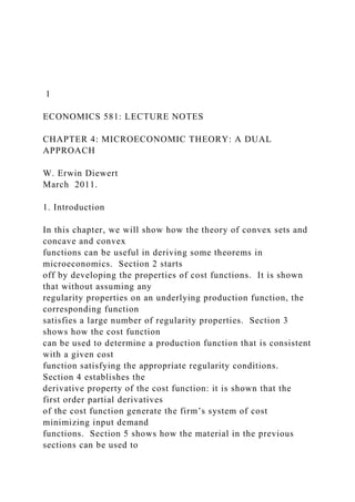
39. Assumption 1 on F: F is continuous from above over the domain
x ≥ 0N.
Assumption 2 on F: F is a nonnegative function with F(0N) = 0
and F(x*) > 0 for at least
one x* > 0N.
As was shown in Theorem 1 above, Assumption 1 is sufficient
to imply that the cost
function C(y,p):
19
(49) C(y,p) ≡ minx {pTx: F(x) ≥ y}
is well defined for all strictly positive input price vectors p >>
0N and all output levels
y∈ Y where Y is the smallest convex set containing the range of
F.
Assumption 2 on F implies that total plant cost will be positive
for positive output y and
positive input price vectors p; that is:
(50) C(y,p) > 0 for y∈ Y, y >
0 and p >> 0N.
The first two assumptions on F are extremely weak. However,
our next assumption,
while reasonably weak, does not always hold.25
Assumption 3 on F: F is such that for every p* >> 0N, a

40. solution y* to the following
average cost minimization problem exists:
(51) miny {C(y,p*)/y: y > 0; y∈ Y} ≡ c(p*).
Figure 3 illustrates the geometry of the average cost
minimization problem (51).
The solid curve in Figure 3 is the graph of the cost C(y,p*) as a
function of y. The slope
of the dashed line in Figure 3 is equal to C(y*,p*)/y* and note
that this line is the line
through the origin that has the lowest slope and is also tangent
to the graph of C(y,p*) as
25 However, one could argue that it will always hold in real
world situations. Eventually, as the target
output level y becomes very large, total costs C(y,p) will
increase at ever increasing rates (due to the
finiteness of world resources) and Assumption 3 will be
satisfied.
y* y
C(y,p*)
Figure 3: The Geometry of Average Cost Minimization
0

41. 20
a function of y. Thus in this case, average plant cost is
uniquely minimized at the output
level y*.
However, one can construct examples of production functions F
where Assumption 3
does not hold. For example, consider the following one output,
one input production
function F defined as follows:
(52) F(x) ≡ (1/2)x2 for 0 ≤ x ≤ 1;
≡ x − (1/2) for x > 1.
If we set the single input price p1 equal to 1, then the cost
function C(y,1) that
corresponds to this F is defined as follows:
(53) C(y,1) ≡ [2y]1/2 for 0 ≤ y ≤ ½;
≡ y + (1/2) for y > ½.
The cost function defined by (53) is graphed in Figure 4.
It can be seen that in this case, average cost is minimized only
asymptotically at an
infinite output level. Hence, there is no finite y* > 0 that
minimizes average cost for this
example and Assumption 3 is not satisfied for this particular
production function.
Let y* solve the average cost minimization problem defined by

42. (51) so that the
minimized average cost is C(y*,p*)/y*. We can regard this
minimized value as a
function of the chosen input price vector p* and in (51), we
have defined this function as
Figure 4: A Cost Function that does not Satisfy Assumption 3
on F
C(y,1)
y
0
21
c(p*). The following result shows that this function c has the
properties of a unit cost
function.
Theorem 8: Diewert (1981; 80): If F(x) satisfies Assumptions 1-
3 listed above, then the
minimum average cost function c(p) defined by (51) is a (i)
positive, (ii) linearly
homogeneous and (iii) concave function of p for p >> 0N.
Proof of (i): Let p* >> 0N and let y* > 0 be a solution to (51).
Then Assumptions 2 and 3
imply that C(y*,p*) > 0 and y* > 0 so that c(p*) = C(y*,p*)/y*
> 0.
Proof of (ii): Let p* >> 0N and let λ* > 0. Then by the
definition of c(λ*p*), we have:

43. (54) c(λ*p*) ≡ miny {C(y,λ*p*)/y: y > 0; y∈ Y}
= miny {λ*C(y, p*)/y: y > 0; y∈ Y}
using the linear
homogeneity property of C(y,p) in p
= λ*miny {C(y, p*)/y: y > 0; y∈ Y} using
λ* > 0
= λ* c(p*)
using (51), the definition of c(p*).
Proof of (iii): Let p1 >> 0N, p2 >> 0N and 0 < λ < 1. Then
using definition (51) for c, it
can be seen that for every y > 0 such that y∈ Y, we have:
(55) C(y,p1)/y ≥ c(p1); C(y,p2)/y ≥ c(p2).
Thus for every y > 0 such that y∈ Y, we have, using the
concavity in prices property of
C(y,p):
(56) C(y,λp1+(1−λ)p2)/y ≥ [λC(y,p1) + (1−λ)C(y,p2)]/y
= λ[C(y,p1)/y] + (1−λ)[C(y,p2)]/y]
≥ λc(p1) + (1−λ)c(p2) using
(55) and λ > 0 and (1−λ) > 0.
Using the definition of c(λp1+(1−λ)p2), we have:
(57) c(λp1+(1−λ)p2) ≡ miny {C(y,λp1+(1−λ)p2)/y: y > 0; y∈ Y}
= C(y*,λp1+(1−λ)p2)/y*
for some y* > 0; y*∈ Y
≥ λc(p1) + (1−λ)c(p2)
using (56) for y = y*. Q.E.D.
Since c(p) is concave over the open domain of definition set,
{p: p >> 0N}, we know that
it is also continuous over this set.26 We also know that the
domain of definition of c can

44. be extended to the nonnegative orthant, Ω ≡ {p: p ≥ 0N} using
the Fenchel (1953; 78)
closure operation and the resulting extension is continuous (and
concave) over Ω.
Now we are in a position to apply the results of problem 5
above. We have just shown
that the c(p) defined by (51) has all of the properties of a unit
cost function and hence,
26We also know that the properties of concavity, linear
homogeneity and positivity are sufficient to imply
that c(p) is nondecreasing in the components of p.
22
there is a constant returns to scale production function f(x) that
is dual to c(p). Using
problem 5, for x >> 0N, define the function g(x) as follows:
(58) g(x) ≡ maxp {c(p): pTx = 1; p ≥ 0N}.
The function g may be used to define the dual to c production
function f as follows:
(59) f(x) ≡ 1/g(x).
It can be shown27 that if we define the unit cost function that
corresponds to the
production function defined by (59), c*(p) say, then this cost
function coincides with the
c(p) that was used in (58), which in turn was defined using the
original cost function
C(y,p) via definition (51); i.e., we have for each p >> 0N:

45. (60) c*(p) ≡ minx {pTx: f(x) ≥ 1} = c(p) ≡ miny {C(y,p)/y: y >
0; y∈ Y}.
As the above material is a bit abstract, we will indicate how the
constant returns to scale
production function f(x) can be constructed from the initially
given plant production
function F(x). For each positive plant output level y > 0, we
can define the corresponding
upper level set L(y) in the usual way:
(61) L(y) ≡ {x : F(x) ≥ y}.
Now define the family of scaled upper level sets M(y) for each
y > 0 with y∈ Y as
follows:
(62) M(y) ≡ {x/y : F(x) ≥ y}.
Thus to determine M(y) for a given y > 0, we find all of the
input vectors x that can
produce at least the output level y using the plant production
function (this is the set L(y))
and then we divide all of those input vectors by the positive
output level y. The
continuity from above property of F implies that the level sets
L(y) and the scaled level
sets M(y) are all nonempty closed sets for each y such that y > 0
and y∈ Y. Now define
the input set U as the union of all of these sets M(y):
(63) U ≡ ∪ y > 0; y∈ Y M(y).
Define the unit output upper level set of the constant returns to
scale production function

46. f as
(64) L ≡ {x : f(x) ≥ 1}.
It turns out that the set U defined by (63) is a subset of the
upper level set L defined by
(64); i.e., we have
27 See Diewert (1974; 110-112).
23
(65) U ⊂ L.
However, it turns out that U is in fact a sufficient statistic for
L; i.e., we can perform
some simple operations on U and transform it into L. We need
to define a couple of set
operations before we do this.
Let S be an arbitrary set in RN. Then the convex hull of S, Con
S, is defined as follows:
(66) Con S ≡ {x : x = λx1 + (1−λ)x2 ; x1∈ S ; x2∈ S and 0 < λ <
1}.
Thus the convex hull of S consists of all of the points belonging
to S plus all of the line
segments joining any two points belonging to S.
The free disposal hull of S, Fdh S, is defined as follows:

47. (67) Fdh S ≡ {x : x ≥ x*; x*∈ S}.
Thus the free disposal hull of S consists of all of the points in S
plus all points that lie
above any point belonging to S.
It turns out that the closure of the free disposal, convex hull of
the set U defined by (63) is
in fact equal to the unit output upper level set L defined by
(64). Thus define U* ≡ Con
U, then define U** ≡ Fdh U* and finally define U*** ≡ Clo
U**. Then U*** = L. The
boundary of the set U can have regions of nonconvexity and
backward bending regions.28
The operation of taking the convex hull of U eliminates these
regions of nonconvexity
and the operation of taking the free disposal convex hull
eliminates any backward
bending regions. Finally, since the union of an infinite number
of closed sets is not
necessarily closed, taking the closure of U** ensures that this
transformed U set is closed.
What is the significance of the unit cost function c defined by
(51) or its dual constant
returns to scale production function f defined by (58) and (59)?
Samuelson (1967; 155-
161) showed that this f represents the asymptotic technology
which is available to the
firm if firm output is large, plants can be replicated and the
plant production function F
satisfies Assumptions 1-3 listed above.
The plant replication idea of Samuelson can be explained as
follows. Let p* >> 0N be
given and let y* > 0 be a solution to the average cost

48. minimization problem (51). For
each positive integer n, define the set of outputs Y(n) as
follows:
(68) Y(n) ≡ {y: (n−1)y* < y ≤ ny*}.
28 Recall Figure 1 above where the boundary of L(y) had
regions of nonconvexity and backward bending
regions.
24
Now consider a situation where a firm has access to the plant
technology production
function F(x) that satisfies Assumptions 1-3 above and has the
dual cost function C(y,p).
Suppose that the firm wants to produce some positive output
level y where y belongs to
the set of outputs Y(n) defined by (68) for some positive integer
n. Then in theory, the
firm could build n plants and have each of them produce 1/n of
the desired output level y.
The firm’s average cost of production using this plant
replication strategy will be equal
to:
(69) cn(y,p*) ≡ C(y/n,p*)/[y/n] ≥ c(p*)
where the inequality in (69) follows from definition (51),which
defined c(p*) as a
minimum.29

49. The following result shows that as the target output level y
becomes large, the average
cost cn(y,p*) using the plant replication strategy approaches the
unit cost c(p*) where the
unit cost function c is dual to the constant returns to scale
production function f defined
earlier by (58) and (59).
Theorem 9: Samuelson (1967; 159), Diewert (1981; 82): As firm
output y becomes large,
average cost using replicable plants cn(y,p*) approaches the
minimum average cost c(p*)
defined by (51); i.e., for every p* >> 0N,
(70) c(p*) = limn→∝ {c
n(y,p*): y∈ Y(n)}.
Proof: If y∈ Y(n), then (n−1)y* < y ≤ ny* or
(71) [(n−1)/n]y* < y/n ≤ y* or
(72) n/y*(n−1) > n/y ≥ 1/y*.
Thus for y∈ Y(n),
(73) cn(y,p*) = C(y/n,p*)/[y/n] using
definition (69)
≤ C(y*,p*)n/y
using (71) and the nondecreasing in y
property of cost functions
< [n/(n−1)]C(y*,p*)/y* using
(72)
= [n/(n−1)] c(p*)
since y* is a solution to the average cost minimization problem
defined by (51). The

50. inequalities (69) and (73) imply that
(74) c(p*) ≤ cn(y,p*) < [n/(n−1)] c(p*).
Taking limits of (74) as n tends to plus infinity gives us (70).
Note that as n increases in
the limit (70), y must also increase in order to remain in the set
Y(n). Q.E.D.
29 We also need y/n∈ Y.
25
The significance of the above result can be explained as
follows. If firm output is large
relative to a minimum average cost output y* when input prices
p* prevail, then the
firm’s total cost function will be approximately equal to yc(p*),
where the unit cost
function c(p) defined by (51) is dual to a well behaved constant
returns to scale
production function f(x). Thus if the firm is behaving
competitively in input markets so
that the firm regards input prices as fixed and beyond their
control, then the firm’s total
demand for inputs can be generated (approximately) by solving
the following cost
minimization problem:
(75) minx {p*Tx: f(x) ≥ y} = yc(p*)
where the asymptotic (or large output) production function f is
positive, linearly

51. homogeneous and concave over the positive orthant,30 even
though the underlying plant
production function F satisfies only Assumptions 1-3.
The geometry of Theorem 9 is illustrated in Figure 5.
In Figure 5, the original plant cost function is C(y,p*) regarded
as a function of y. The
straight line through the origin is tangent to this curve at the
minimum average cost
output level y*. Note that this straight line represents the
minimum average cost that is
attainable for this particular plant technology. The function
c2(y,p*) ≡ 2C(y/2,p*) can be
30 Production functions that have these properties are often
called neoclassical production functions. Of
course, the function f can be extended in a continuous manner
to the nonnegative orthant using the Fenchel
closure operation.
Costs
Figure 5: The Asymptotic Cost Function
0 y* 2y* 3y*
y
C(y,p*) c2(y,p*)
c3(y,p*)
Envelope Average

52. Cost
Asymptotic
Marginal Cost
26
graphed using the original cost curve C(y,p*) and so can the
function c3(y,p*) ≡
3C(y/3,p*). The dashed line labelled as the envelope average
cost is the minimum
average cost that corresponds to the three total cost curves that
appear in Figure 5.
Obviously, if the firm can replicate plants, this dashed line will
represent the minimum
average cost of producing any output level up to 3y*. Note that
as the target output level
y increases, this scalloped average cost line gets closer and
closer to the straight line that
is labelled as the asymptotic marginal cost line. Thus if (a)
firm output y is large relative
to the smallest minimum average cost output level y*, (b) the
firm behaves competitively
in input markets and (c) plants can be replicated without
difficulties, then we can closely
approximate the firm’s behavior in input markets by assuming
that it possesses a constant
returns to scale production function f defined above by (58) and
(59), rather than the
nonconstant returns to scale plant production function F.
7. Aggregation and the Size of Input Price Elasticities of
Demand

53. A great many problems in cost benefit analysis and applied
economics in general hinge
on the size of various elasticities of demand or supply. In this
section, we will show that
increasing the degree of aggregation in a production model will
generally lead to
elasticities of derived demand that are smaller in magnitude
than the average of the micro
elasticities of demand in the aggregate.
Consider a one output technology, y = F(z,x), that uses
combinations of M + N inputs, z
≥ 0M and x ≥ 0N, to produce output y ≥ 0. Let the cost function
that corresponds to this
technology be the twice differentiable function, C(y,w,p),
defined in the usual way as
follows:
(76) C(y,w,p) ≡ minz,x {wTz + pTx: F(z,x) ≥ y}
where y > 0 is the target output level and w >> 0M and p >> 0N
are strictly positive input
price vectors. This cost function will satisfy the regularity
conditions in Theorem 1
above. The two sets of cost minimizing input demand
functions, z(y,w,p) and x(y,w,p),
can be obtained by using Shephard’s Lemma:
(77) z(y,w,p) = ∇ wC(y,w,p) ;
(78) x(y,w,p) = ∇ pC(y,w,p).
We now introduce the assumption that the prices in the vector w
move proportionally
over time31 (or space if we are in a cross sectional context);
i.e., we assume that

54. (79) w = αp0 ; α ≡ [α1,…,αM]T >> 0M.
31 This is the framework used by Hicks (1946; 312-313) in his
Composite Commodity Aggregation
Theorem: “Thus we have demonstrated mathematically the very
important principle, used extensively in
the text, that if the prices of a group of goods change in the
same proportion, that group of goods behaves
just as if it were a single commodity.”
27
We now construct an aggregate of the z inputs. Usually, we set
one of the components of
α equal to unity (e.g., set α1 = 1) so that the remaining αm tell
us how many units of input
m are equivalent to one unit of input 1 in the z group of inputs.
The “quantity” of the z
aggregate, x0, is defined in practice by deflating observed
expenditure on the z inputs by
the numeraire price p0; i.e., we have
(80) x0(y,w,p) ≡ ∑m=1M wmzm(y,w,p)/p0
= ∑m=1M p0αmzm(y,αp0,p)/p0
using (79)
= αTz(y,αp0,p).
To see how Hicks’ Aggregation Theorem works in this context,
we use the aggregation
vector α, which appears in (79) in order to construct an
aggregate input requirements
function,32 G(y,x,α), as follows:33

55. (81) x0 = G(y,x,α) ≡ minz {αTz: F(z,x) ≥ y}.
The above aggregate input requirements function G can be used
in order to define the
following aggregate cost function, C*:
(82) C*(y,p0,p) ≡ {p0x0 + pTx: x0 = G(y,x,α)}
= minx {p0G(y,x,α) + pTx} using
the constraint to eliminate x0
= minx {p0[minz {αTz: F(z,x) ≥ y}] + pTx}
using (81)
= minx,z {p0αTz + pTx: F(z,x) ≥ y}
using p0 > 0
= minx,z {wTz + pTx: F(z,x) ≥ y}
using (79)
≡ C(y,w,p)
using (76).
The string of equalities in (82) shows that if (z*,x*) solves the
original micro cost
minimization problem defined by (76), then x0* ≡ αTz* and x*
solve the macro cost
minimization problem defined by the first line in (82). Thus if
the z input prices vary in
strict proportion over time, then these inputs can be aggregated
using the construction in
(80), and the resulting x0 aggregate will obey the usual
properties of an input demand
function that is consistent with cost minimizing behavior. This
is a version of Hicks’
(1946; 312-313) Aggregation Theorem.
We now want to explore the relationship of the price elasticities
of demand for the
aggregate input compared to the underlying micro cross

56. elasticities of demand.
The microeconomic matrices of input price elasticities of
demand can be defined as
follows:34
32 An input requirements function, x0 = g(y,x), gives the
minimum amount of an input x0 that is required to
produce the output level y given that the vector of other inputs
x is available for the production function
constraint y = f(x0,x). Thus g is a (conditional on x) inverse
function for y regarded as a function of x0,
holding x constant. Input requirements functions were studied
by Diewert (1974c).
33 If there is no z ≥ 0M such that F(z,x) ≥ y, then G(x,y,α) is
defined to equal plus infinity.
34 All of these elasticities are evaluated at an initial point
(y,w,p).
28
(83) Exp ≡ [enk]
n = 1,…,N ; k = 1,…,N
≡ [(pk/xn)∂xn(y,w,p)/∂pk]
= [(pk/xn)∂2C(y,w,p)/∂pn∂pk]
using (78)
= −1∇ 2ppC(y,w,p)
where and denote N by N diagonal matrices with the positive
elements of the x and p
vectors running down the main diagonal respectively;

57. (84) Ezw ≡ [emk]
m = 1,…,M ; k = 1,…,M
≡ [(wk/zm)∂zm(y,w,p)/∂wk]
= [(wk/zm)∂2C(y,w,p)/∂wm∂wk]
using (77)
= −1∇ 2wwC(y,w,p)
where and denote M by M diagonal matrices with the positive
elements of the z
and w vectors running down the main diagonal respectively;
(85) Ezp ≡ [emn]
m = 1,…,M ; n = 1,…,N
≡ [(pn/zm)∂zm(y,w,p)/∂pn]
= [(pn/zm)∂2C(y,w,p)/∂wm∂pn]
using (77)
= −1∇ 2wpC(y,w,p) .
Using the linear homogeneity property of the cost function
C(y,w,p) in the components of
(w,p), it can be shown that the elasticity matrices Ezw and Ezp
satisfy the following
restrictions:35
(86) Ezw1M + Ezp1N = −1∇ 2wwC(y,w,p) 1M +
−1∇ 2wpC(y,w,p) 1N
using (84) and (85)
= −1{∇ 2wwC(y,w,p)w + ∇ 2wpC(y,w,p)p}
= −1{0M}
using Part 2 of Euler’s Theorem
on homogeneous functions
= 0M.
Thus the elements in each row of the M by M+N elasticity
matrix [Ezw,Ezp] sum to zero.

58. Now we are ready to calculate the price elasticity of demand of
the input aggregate x0
with respect to its own price p0. We first differentiate the last
equation in (80) with
respect to p0:
(87) ∂x0(y,αp0,p)/∂p0 = ∑m=1M αm ∑k=1M
[∂zm(y,αp0,p)/∂wk][∂(αkp0)/∂p0]
= ∑m=1M αm ∑k=1M
[∂zm(y,αp0,p)/∂wk]αk
= ∑m=1M ∑k=1M
αm[∂2C(y,αp0,p)/∂wm∂wk]αk using (77)
35 Notation: 1M and 1N are vectors of ones of dimension M and
N respectively.
29
= ∑m=1M ∑k=1M
αm[∂2C(y,w,p)/∂wm∂wk]αk using (79)
= αT∇ 2wwC(y,w,p)α
≤ 0
where the last inequality follows from the negative
semidefiniteness of ∇ 2wwC(y,w.p),
which in turn follows from the fact that C(y,w,p) is concave in
the components of w.
Thus the own price elasticity of demand for the input aggregate
will be negative or 0.
Now calculate the price elasticity of demand of the input
aggregate x0 with respect to the
prices pn for n = 1,…,N. We first differentiate the last equation

59. in (80) with respect to pn:
(88) ∂x0(y,αp0,p)/∂pn = ∑m=1M αm ∂zm(y,αp0,p)/∂pn
for n = 1,…,N
= ∑m=1M αm∂2C(y,w,p)/∂wm∂pn
using (77)
= αT∇ 2wpC(y,w,p)en
where en is an N dimensional unit vector; i.e., it has all
elements equal to 0 except that the
nth component is equal to 1.
We are ready to convert the derivatives defined by (87) and (88)
into the own and cross
price elasticities of demand for the aggregate, ε00 and ε0n for
n = 1,…,N:
(89) ε00 ≡ [p0/x0][∂x0(y,αp0,p)/∂p0]
= [p0/x0][αT∇ 2wwC(y,w,p)α]
using (87)
= p0αT∇ 2wwC(y,w,p)p0α/p0x0
= wT∇ 2wwC(y,w,p)w/p0x0
using (79)
= wT∇ 2wwC(y,w,p)w/ ∑m=1M wmzm(y,w,p)
using (80)
= wT −1∇ 2wwC(y,w,p)w/wTz
since −1 = IM
= wT −1∇ 2wwC(y,w,p) 1M/wTz
since w = 1M
= wT Ezw1M/wTz
using (84)
= sT Ezw1M
≤ 0
where the vector of expenditure shares on the components of z
is defined as sT ≡

60. [s1,…,sM] where
(90) sm ≡ wmzm(y,w,p)/wTz(y,w,p)
for m = 1,…,M.
The inequality in (89) follows from (87), ∂x0(y,αp0,p)/∂p0 ≤ 0,
and the positivity of p0
and x0.
Converting the derivatives in (88) into elasticities leads to the
following equations:
(91) ε0n ≡ [pn/x0][∂x0(y,αp0,p)/∂pn]
for n = 1,…,N
= [pn/x0][αT∇ 2wpC(y,w,p)en]
using (88)
= p0αT∇ 2wpC(y,w,p)pnen/p0x0
30
= wT∇ 2wpC(y,w,p)pnen/p0x0
using (79)
= wT∇ 2wpC(y,w,p)pnen/ ∑m=1M wmzm(y,w,p)
using (80)
= wT −1∇ 2wpC(y,w,p)pnen /wTz
since −1 = IM
= wT −1∇ 2wpC(y,w,p) en /wTz
since pnen = en
= wT Ezpen/wTz
using (85)
= sT Ezpen .
Using the above formulae for the ε0n, we can compute the sum
of the ε0n as follows:

61. (92) ∑n=1N ε0n = ∑n=1N sT Ezpen
= sTEzp1N .
Now use (89) and (92) in order to compute the sum of all of the
price elasticities of
demand of the input aggregate with respect to its own price p0
as well as the other input
prices outside of the aggregate, p1,…,pN:
(93) ε00 + ∑n=1N ε0n = sTEzw1M + sTEzp1N
= sT{Ezw1M + Ezp1N}
= sT {0M}
using (86)
= 0.
Using (89), we have ε00 ≤ 0. Hence (93) implies that
(94) ∑n=1N ε0n = − ε00 ≥ 0.
Consider the cross elasticity of demand of the input aggregate
with the input price pn for
some n = 1,…,N. Using (91), we have
(95) ε0n = ∑m=1M smemn ≤ ∑m=1M sm |emn|
for n = 1,…,N
where the inequality follows since the shares sm are always
positive and the cross
elasticity of demand for the micro input zm with respect to the
price pn, emn, is always
equal to or less than its absolute value, |emn|. Hence if any of
the inputs m in the group of
inputs being aggregated (the zm) are complementary to the
input xn, then the
corresponding emn will be negative and the inequality (95) will

62. be strict for that n.
In general, it can be seen that the cross elasticities of aggregate
input demand ε0n are
weighted averages of the micro cross elasticities of demand
emn. If all of these micro
cross elasticities of demand are nonnegative (so that there are
no complementary input
pairs between the z and x groups of inputs), then it can be seen
that the aggregate cross
elasticities of demand ε0n will be weighted averages of the emn
and will be roughly
comparable in magnitude to the average magnitude of the emn.
However, the greater the
degree of complementarity between the z and x groups of
inputs, the greater will be the
reduction in the magnitudes of the ε0n compared to the
magnitudes of the emn, which are
31
the absolute values |emn|.36 How likely is complementarity in
empirical applications?
Most empirical applications of production theory impose
substitutability between every
pair of inputs and so it is frequently thought that
complementarity is a somewhat rare
phenomenon. However, if flexible functional form techniques
are used, then typically, if
the number of inputs is greater than 3, complementarity is
encountered.37
Finally, we compare the magnitude of the own price elasticity
of demand of the input

63. aggregate, ε00, with the weighted average of the micro own
price elasticities of demand in
the aggregate, ∑m=1M smemm. Using (89), we have ε00 ≤ 0
and the micro own price
elasticities of demand, emm, are also nonpositive.38 Hence
(96) 0 ≤ − ε00
= − ∑m=1M ∑k=1M sm emk
using (89)
= − ∑m=1M sm emm − ∑m=1M ∑k=1M m≠k sm emk
< − ∑m=1M sm emm
where the inequality follows provided that
(97) ∑m=1M ∑k=1M m≠k sm emk > 0.
The strict inequality in (96) says that the magnitude (or absolute
value) of ε00 is smaller
than the magnitude of the weighted average of the micro own
price elasticities of demand
in the input aggregate, ∑m=1M sm emm. However the strict
inequality in (96) will hold only
if the strict inequality in (97) holds. We cannot guarantee that
(97) will hold but it is very
likely that it will hold. In particular, (97) will hold if all of the
input pairs in the z group
of inputs are substitutes or are unrelated so that in this case,
emk ≥ 0 for all m ≠ k.39
We can summarize the above results as follows: if we estimate
price elasticities of input
demand for an aggregated model and compare the resulting
elasticities with the
elasticities obtained from the more disaggregated model, there
will be a strong tendency
for the elasticities in the aggregated model to be smaller in

64. magnitude than those in the
disaggregated model.40
36 This point was made by Diewert (1974b; 16) many years ago
in the elasticity of substitution context:
“Taking a weighted average of both positive and negative micro
elasticities of substitution σm
n will tend to
give rise to aggregate elasticities of substitution which are
considerably smaller in magnitude than an
average of the absolute values of the micro elasticities of
substitution.”
37 For example, see the 4 input evidence on the incidence of
complementarity tabled in Diewert and Wales
(1987; 63).
38 This follows from the fourth characterization of concavity
and the fact that C(y,w,p) is concave in w.
39 Strictly speaking, we need at least one input pair to be
substitutes so that emk > 0 for this pair of inputs
and the other input pairs could be unrelated.
40 For the 4 input models estimated in Diewert and Wales
(1987; 63), the input price elasticities were all
less than 1.2 in magnitude. For the 8 output and input model
estimated by Diewert and Wales (1992; 716-
717), all of the tabled price elasticities were less than 3.43 in
magnitude. For the 12 output and input model
estimated by Diewert and Lawrence (2002; 154), all of the
tabled price elasticities (excluding inventory
change which was very volatile) were less than 8.99 in
magnitude.

65. 32
In actual empirical examples, the strict proportionality
assumptions made in (79) will not
hold exactly and the aggregates will be constructed using an
index number formula that
will be consistent with the assumptions (79) if they happen to
hold.41 However, even if
the assumption of price proportionality (79) holds only
approximately, empirical
evidence suggests that elasticities do decline in magnitude as
the degree of aggregation
increases. We conclude with a quotation that summarizes some
early empirical evidence
on this phenomenon:42
“Conversely, as we disaggregate, we can expect to encounter
increasingly large elasticities of substitution.
Two recent papers confirm this statement. Berndt and
Christensen (1974) in their ‘two types of labour, one
type of capital” disaggregation of US manufacturing industries
found that the mean partial elasticities of
substitution were 7.88 (between blue and white collar workers),
3.72 (between blue collar workers and
capital) and −3.77 (between white collar workers and capital).
However, when they fitted a model which
aggregated the two types of labour into a single labour factor,
they found that the aggregate labour-capital
elasticity of substitution was approximately 1.42, which is
considerably smaller that an average of the three
‘micro’ elasticities of substitution. Similarly, Woodland (1972)
found partial elasticities of substitution in
Canadian manufacturing ranging from −11.16 to 2.18 in his
‘four types of capital, one type of labour’
disaggregated results, but he found that the aggregate capital-
labour elasticity of substitution was only

66. 0.39.”
W.E. Diewert (1974b; 16).
Problems
15. The N by M matrix of cross elasticities of demand of the x
inputs with respect to the
prices of the z inputs can be defined as follows:
(i) Exw ≡ [enm]
n = 1,…,N ; m = 1,…,M
≡ [(wm/xn)∂xn(y,w,p)/∂wm]
= [(wm/xn)∂2C(y,w,p)/∂pn∂wm]
using (78)
= −1∇ 2pwC(y,w,p) .
Show that the matrices of elasticities Exp defined by (83) and
Exw defined by (i) above
satisfy the following restriction:
(ii) Exp1N + Exw1M = 0N.
16. Suppose that the N+M by N+M symmetric matrix C is
negative semidefinite. Write
the matrix C in partitioned form as follows:
(i)
41 In fact, it is useful to aggregate commodities whose prices
move almost proportionally over time since
the resulting aggregates will be approximately consistent with
Hicks’ Aggregation Theorem.

67. 42 Part (b) of problem 17 below shows that elasticities of
substitution are equal to price elasticities of
demand divided by cost shares and hence will be considerably
larger than price elasticities of demand so
that the numbers in the quotation below are a bit misleading.
33
where C11 is N by N and symmetric and C22 is M by M and
symmetric. Show that C11
and C22 are also negative semidefinite matrices.
17. Let C(y,p) be a twice continuously differentiable cost
function that satisfies the
regularity conditions listed in Theorem 1 in section 2 above.
By Shephard’s Lemma, the
input demand functions are given by
(i) xn(y,p) = ∂C(y,p)/∂pn > 0; n = 1,…,N.
The Allen (1938; 504) Uzawa (1962) elasticity of substitution
σnk between inputs n and k
is defined as follows:
(ii) σnk(y,p) ≡
{C(y,p)∂2C(y,p)/∂pn∂pk}/{[∂C(y,p)/∂pn][∂C(y,p)/∂pk]} 1 ≤
n,k ≤ N
= {C(y,p)∂2C(y,p)/∂pn∂pk}/xn(y,p) xk(y,p)
using (i).
Define Σ ≡ [σnk(y,p)] as the N by N matrix of elasticities of
substitution.
(a) Show that Σ has the following properties:

68. (iii) Σ = ΣT ;
(iv) Σ is negative semidefinite and
(v) Σs = 0N
where s ≡ [s1,…,sN]T is the vector of cost shares; i.e., sn ≡ pn
xn(y,p)/C(y,p) for n =
1,…,N. Now define the N by N matrix of cross price elasticities
of demand E in a
manner analogous to definition (83) above:
(vi) E ≡ [enk]
n = 1,…,N ; k = 1,…,N
≡ [(pk/xn)∂xn(y,p)/∂pk]
= [(pk/xn)∂2C(y,p)/∂pn∂pk]
using (i)
= −1∇ 2ppC(y,p) .
(b) Show that E = Σ where is an N by N diagonal matrix with
the elements of the
share vector s running down the main diagonal.
18. Suppose a firm’s cost function has the following Constant
Elasticity of Substitution
(CES) functional form:43
(i) C(y,p1,…,pN) ≡ ky[∑n=1N αnpnr]1/r; k > 0; r ≤ 1, r ≠
0; αn > 0 and ∑n=1N αn = 1.
Thus the cost function is equal to a positive constant k times the
output level y times a
mean of order r. From the chapter on inequalities, we know that
C(y,p) is a concave
function of p provided that r is equal to or less than one. Show
that

69. 43 This functional form was introduced into the production
literature by Arrow, Chenery, Minhas and
Solow ((1961).
34
(ii) σnk(y,p) = −(r−1) for all n,k such that n ≠ k
where σnk(y,p) is the elasticity of substitution between inputs n
and k defined above in
problem 17, part (ii). Comment: This problem shows why the
CES functional form is
unsatisfactory if the number of inputs N exceeds two, since it is
a priori unlikely that all
elasticities of substitution between every pair of inputs would
equal the same number.
8. The Application of Cost Functions to Consumer Theory
The cost function and production function framework described
in the previous sections
can be readily adapted to the consumer context: simply replace
output y by utility u,
reinterpret the production function F as a utility function,
reinterpret the input vector x as
a vector of commodity demands and reinterpret the vector of
input prices p as a vector of
commodity prices. With these changes, the producer’s cost
minimization problem (1)
becomes the following problem of minimizing the cost or
expenditure of attaining a given
level of utility u:

70. (98) C(u,p) ≡ minx {pTx : F(x) ≥ u }.
If the cost function is differentiable with respect to the
components of the commodity
price vector p, then Shephard’s (1953; 11) Lemma applies and
the consumer’s system of
commodity demand functions as functions of the chosen utility
level u and the
commodity price vector p, x(u,p), is equal to the vector of first
order partial derivatives of
the cost or expenditure function C(u,p) with respect to the
components of p:
(99) x(u,p) = ∇ pC(u,p).
The demand functions xn(u,p) defined in (99) are known as
Hicksian44 demand functions.
Thus it seems that we can adapt the theory of cost and
production functions used in
section 2 above in a very straightforward way, replacing output
y by utility u and
reinterpreting all of our previous results. However, there is a
problem: the output level y
is an observable variable but the corresponding utility level u is
not observable!
However, this problem can be solved (but as we will see, some
of the details are rather
complex). We need only equate the cost function C(u,p) to the
consumer’s observable
expenditure in the period under consideration, Y say, and solve
the resulting equation for
u as a function of Y and p, say u = g(Y,p). Thus u = g(Y,p) is
the u solution to the
following equation:

71. (100) C(u,p) = Y
44 See Hicks (1946; 311-331).
35
and the resulting solution function u = g(Y,p) is the consumer’s
indirect utility function.
Now replace the u in the system of Hicksian demand functions
(99) by g(Y,p) and we
obtain the consumer’s system of (observable) market demand
functions:
(101) d(Y,p) = ∇ pC(g(Y,p),p).
We illustrate the above procedure for the generalized Leontief
cost function defined by
(27) above. For this functional form, equation (100) becomes:
(102) u ∑i=1N∑j=1N bij pi1/2 pj1/2 = Y ; (bij
= bji for all i and j)
and the u solution to this equation is:
(103) u = g(Y,p) = Y/[∑i=1N∑j=1N bij pi1/2 pj1/2].
The Hicksian demand functions for the C(u,p) defined by the
left hand side of (102) are:
(104) xn(u,p) ≡ ∂C(u,p)/∂pn = [∑j=1N bnj (pj/pn)1/2]u ;
n = 1,…,N.

72. Substituting (103) into (104) leads to the following system of
market demand functions:
(105) dn(Y,p) = [∑j=1N bnj (pj/pi)1/2] Y/[∑i=1N∑j=1N bij
pi1/2 pj1/2] ; n = 1,...,N.
Equations (105) can be used as the basis for the econometric
estimation of preferences.
Suppose that we have collected data on the quantities xnt
purchased over T time periods
for a household as well as the corresponding commodity prices
pnt. Then we can define
period t “income”45 or expenditure on the n commodities as Yt:
(106) Yt ≡ ∑n=1N pntxnt ;
t = 1,…,T.
Evaluating (105) at the period t data and adding a stochastic
error term ent to equation n in
(105) for n = 1,...,N leads to the following system of estimating
equations:
(107) xnt = [∑j=1N bnj (pjt/pnt)1/2] Yt/[∑i=1N∑j=1N bij
(pit)1/2 (pjt)1/2]+ ent; t = 1,...,T; n = 1,...,N.
Not all N equations in (107) can have independent error terms
since if we multiply both
sides of equation n in (107) by pnt and sum over n, we obtain
the following equation:
(108) ∑n=1N pntxnt = Yt + ∑n=1N pntent.
Using (106), we find that the period t errors ent satisfy the
following linear restriction
exactly:

73. 45 Strictly speaking, a household’s income will also include
savings in addition to expenditures on current
goods and services.
36
(109) ∑n=1N pntent = 0 ;
t = 1,…,T.
There is one other factor that must be taken into account in
doing an econometric
estimation of preferences using the system of estimation
equations (107). Note that if we
multiply all of the bij parameters by the positive number λ, the
right hand sides of each
equation in (107) will remain unchanged; i.e., the demand
functions are homogeneous of
degree 0 in the bij parameters. Thus these parameters will not
be identified as matters
stand. Hence, it will be necessary to impose a normalization on
these parameters. One
normalization that is frequently used in applied economics is to
set unit cost46 equal to 1
for some set of reference prices p0 say.47 Thus we impose the
following normalization on
the bij:
(110) 1 = c(p0) = ∑i=1N∑j=1N bij (pi0)1/2 (pj0)1/2.
Equation (110) can be used to solve for say b11 in terms of the
other bij and then this

74. equation can be used to eliminate b11 from the N−1 independent
estimating equations in
(107) and the remaining parameters can be estimated using
nonlinear regression
techniques.
The technique suggested above for the econometric estimation
of preferences is a special
case of the following general strategy: (i) Assume that the
consumer’s preferences can be
represented by the cost function C(u,p) that has the following
form:
(111) C(u,p) = uc(p)
where c(p) is a suitable differentiable unit cost function. (ii)
Differentiate (111) with
respect to the components of the commodity price vector p to
form the following system
of Hicksian demand functions:
(112) x(u,p) = u ∇ pc(p) .
(iii) Equate cost uc(p) to expenditure or income Y and solve for
u as a function of Y and
p to get the consumer’s indirect utility function u = g(y,p):
(113) u =Y/c(p).
(iv) Substitute (113) into the right hand side of (112) in order to
obtain the following
system of consumer demand functions:
(114) d(Y,p) = ∇ pc(p)Y/c(p).
(v) Finally, impose the normalization (110), c(p0) = 1, in order

75. to identify all of the
unknown parameters in (114).
46 The Generalized Leontief cost function defined by (27) has
the form C(u,p) = uc(p) where c(p) ≡ C(1,p).
47 Usually, p0 is taken to be p1, the vector of prices that
prevailed in the base period.
37
Unfortunately, there is a problem with the above strategy for
estimating a consumer’s
preferences. The problem is the same one that occurred in
problem 14 above; with the
nth consumer demand function, dn(Y,p) defined by the nth
equation in (114), we find that
all income elasticities of demand are equal to one; i.e., we have:
(115) [Y/dn(Y,p)]∂dn(Y,p)/∂Y = 1 ;
n = 1,…,N.
But (115) contradicts Engel’s Law, which says that the income
elasticity of demand for
food is less than one.
In the following two sections, we show how this problem of
unitary income elasticities
can be solved.
9. Flexible Functional Forms and Nonunitary Income
Elasticities of Demand

76. We first define what it means for a unit cost function, c(p), to
be a flexible functional
form. Let c*(p) be an arbitrary unit cost function that satisfies
the appropriate regularity
conditions on unit cost functions and in addition, is twice
continuously differentiable
around a point p* >> 0N. Then we say that a given unit cost
function c(p) that is also
twice continuously differentiable around the point p* is flexible
if it has enough free
parameters so that the following 1 + N + N2 equations can be
satisfied:
(116) c(p*) = c*(p*) ;
(117) ∇ c(p*) = ∇ c*(p*) ;
(118) ∇ 2c(p*) = ∇ 2c*(p*).
Thus c(p) is a flexible functional form if it has enough free
parameters to provide a
second order Taylor series approximation to an arbitrary unit
cost function.
At first glance, it looks like c(p) will have to have at least 1 + N
+ N2 independent
parameters in order to be able to satisfy all of the equations
(116)-(118). However, since
both c and c* are assumed to be twice continuously
differentiable, Young’s Theorem in
calculus implies that ∂2c(p*)/∂pi∂pj = ∂2c(p*)/∂pj∂pi for all i ≠
j (and of course, the same
equations hold for the second order partial derivatives of c*(p)
when evaluated at p = p*).
Thus the N2 equations in (118) can be replaced with the
following N(N+1)/2 equations:
(119) ∂2c(p*)/∂pi∂pj = ∂2c*(p*)/∂pj∂pi for 1 ≤ i ≤ j ≤ N.

77. Another property that both unit cost functions must have is
homogeneity of degree one in
the components of p. By part 1 of Euler’s Theorem on
homogeneous functions, c and c*
satisfy the following equations:
(120) c(p*) = p*T∇ c(p*) and c*(p*) = p*T∇ c*(p*).
38
Thus if c and c* satisfy equations (117), then using (120), we
see that c and c*
automatically satisfy equation (116). By part 2 of Euler’s
Theorem on homogeneous
functions, c and c* satisfy the following equations:
(121) ∇ 2c(p*)p* = 0N and ∇ 2c*(p*)p* = 0N.
This means that if we have ∂2c(p*)/∂pi∂pj = ∂2c*(p*)/∂pi∂pj for
all i ≠ j, then equations
(121) will imply that ∂2c(p*)/∂pj∂pj = ∂2c*(p*)/∂pj∂pj as well,
for j = 1,…,N.
Summarizing the above material, if c(p) is linearly
homogeneous, then in order for it to
be flexible, c(p) needs to have only enough parameters so that
the N equations in (117)
can be satisfied and so that the following N(N−1)/2 equations
can be satisfied:
(122) ∂2c(p*)/∂pj∂pj = ∂2c*(p*)/∂pi∂pj ≡ cij* for 1 ≤ i < j ≤ N.

78. Thus in order to be flexible, c(p) must have at least N +
N(N−1)/2 = N(N+1)/2
independent parameters.
Now consider the Generalized Leontief unit cost function
defined as follows:48
(123) c(p) ≡ ∑i=1N∑j=1N bij pi1/2 pj1/2 ; bij =
bji for all i and j.
Note that there are exactly N(N+1)/2 independent bij parameters
in the c(p) defined by
(123). For this functional form, the N equations in (117)
become:
(124) ∂c(p*)/∂pn = ∑j=1N bnj (pj*/pn*)1/2 = ∂c*(p*)/∂pn ≡ cn*
; n = 1,…,N.
The N(N−1)/2 equations in (122) become:
(125) (1/2)bij /(pi*pj*)1/2 = cij* ;
1 ≤ i < j ≤ N.
However, it is easy to solve equations (125) for the bij:
(126) bij = 2cij*(pi*pj*)1/2 ;
1 ≤ i < j ≤ N.
Once the bij for i < j have been determined using (126), we set
bji = bij for i < j and finally
the bii are determined using the N equations in (124).
The above material shows how we can find a flexible functional
form for a unit cost
function49. We now turn our attention to finding a flexible
functional form for a general

79. cost function C(u,p). Let C*(u,p) be an arbitrary cost function
that satisfies the
appropriate regularity conditions on cost functions listed in
Theorem 1 above and in
48 We no longer restrict the bij to be nonnegative.
49 This material can be adapted to the case where we want a
flexible functional form for a linearly
homogeneous utility or production function f(x): just replace p
by x and c(p) by f(x).
39
addition, is twice continuously differentiable around a point
(u*,p*) where u* > 0 and p*
>> 0N. Then we say that a given cost function C(u,p) that is
also twice continuously
differentiable around the point (u*,p*) is flexible if it has
enough free parameters so that
the following 1 + (N+1) + (N+1)2 equations can be satisfied:
(127) C(u*,p*) = C*(u*,p*) ; (1
equation)
(128) ∇ pC(u*,p*) = ∇ pC*(u*,p*) ; (N
equations)
(129) ∇ 2ppC(u*,p*) = ∇ 2ppC*(u*,p*) ; (N2
equations)
(130) ∇ uC(u*,p*) = ∇ uC*(u*,p*) ; (1
equation)
(131) ∇ 2puC(u*,p*) = ∇ 2puC*(u*,p*) ; (N
equations)
(132) ∇ 2upC(u*,p*) = ∇ 2upC*(u*,p*) ; (N
equations)

80. (133) ∇ 2uuC(u*,p*) = ∇ 2uuC*(u*,p*) (1
equation).
Equations (127)-(129) are the counterparts to our earlier unit
cost equations (116)-(118).
As was the case with unit cost functions, equation (127) is
implied by the linear
homogeneity in prices of the cost functions and Part 1 of
Euler’s Theorem on
homogeneous functions. Young’s Theorem on the symmetry of
cross partial derivatives
means that the lower triangle of equations in (129) is implied by
the equalities in the
upper triangle of both matrices of partial derivatives. Part 2 of
Euler’s Theorem on
homogeneous functions implies that if all the off diagonal
elements in both matrices in
(129) are equal, then so are the diagonal elements. Hence, in
order to satisfy all of the
equations in (127)-(129), we need only satisfy the N equations
in (128) and the N(N−1)/2
in the upper triangle of equations (129). Young’s Theorem
implies that if equations
(131) are satisfied, then so are equations (132). However,
Euler’s Theorem on
homogeneous functions implies that
(134) ∂C(u*,p*)/∂u = p*T∇ 2puC(u*,p*) = p*T∇ 2puC*(u*,p*) =
∂C*(u*,p*)/∂u .
Hence, if equations (131) are satisfied, then so is the single
equation (130). Putting this
all together, we see that in order for C to be flexible, we need
enough free parameters in
C so that the following equations can be satisfied:

81. • Equations (128); N equations;
• The upper triangle in equations (129); N(N−1)/2 equations;
• Equations (131); N equations; and
• Equation (133); 1 equation.
Hence, in order for C to be a flexible functional form, it will
require a minimum of 2N +
N(N−1)/2 +1 = N(N+1)/2 + N +1 parameters. Thus a fully
flexible cost function, C(u,p),
will require N + 1 additional parameters compared to a flexible
unit cost function, c(p).
Suppose the unit cost function is the Generalized Leontief unit
cost function c(p) defined
by (123) above. We now show how terms can be added to it in
order to make it a fully
flexible cost function. Thus define C(u,p) as follows:
(135) C(u,p) ≡ uc(p) + bTp + (1/2)a0αTpu2
40
where bT ≡ [b1,…,bN] is an N dimensional vector of new
parameters, a0 is a new
parameter and αT ≡ [α1,…,αN] > 0N is a vector of
predetermined parameters.50 Using
(135) as our C, equations (128), (129), (131) and (133) become:
(136) u*∇ pc(p*) + b + (1/2)a0αu*2 = ∇ pC*(u*,p*) ;
(137) u*∇ 2ppc(p*) = ∇ 2ppC*(u*,p*) ;
(138) ∇ pc(p*) + a0αu* = ∇ 2puC*(u*,p*) ;
(139) a0αTp* = ∇ 2uuC*(u*,p*) .

82. Use equations (137) in order to determine the bij for i ≠ j. Use
(139) in order to determine
the single parameter a0. Use equations (138) in order to
determine the bii. Finally, use
equations (136) in order to determine the parameters bn in the b
vector. Thus the cost
function C(u,p) defined by (135), which uses the Generalized
Leontief unit cost function
c(p) defined by (123) as a building block, is a parsimonious
flexible functional form for a
general cost function.
In fact, it is not necessary to use the Generalized Leontief unit
cost function in (135) in
order to convert a flexible functional form for a unit cost
function into a flexible
functional form for a general cost function. Let c(p) be any
flexible functional form for a
unit cost function and define C(u,p) by (135). Use equation
(139) to determine the
parameter a0. Once a0 has been determined, equations (137)
and (138) can be used to
determine the parameters in the unit cost function c(p).51
Finally, equations (136) can be
used to determine the parameters in the vector b.
Obviously, the material in this section can be applied to the
problems involved in
estimating a flexible cost function in the production context:
simply replace utility u by
output y and reinterpret the commodity price vector p as an
input price vector.
Differentiating (135) leads to the following system of
estimating equations, where x(y,p)
= ∇ pC(y,p) is the producer’s system of cost minimizing input

83. demand functions:
(140) x(y,p) = y∇ c(p) + b + (1/2)a0αy2.
In order to obtain estimating equations for the general cost
function defined by (135),
there are some normalization issues that need to be discussed.
We do this in the
following section.
10. Money Metric Utility Scaling and Other Methods of
Cardinalizing Utility
50 The parameter a0 could be set equal to 1 and the vector of
parameters α could be estimated
econometrically. We have defined the cost function C in this
manner so that it has the minimal number of
parameters required in order to be a flexible functional form.
Thus it is a parsimonious flexible functional
form.
51 It can be seen that equations (137) and (138) have the same
structure as equations (117) and (118).
Hence if c(p) has enough free parameters to satisfy (117) and
(118), then it has enough free parameters to
satisfy (137) and (138) once a0 has been determined.
41
Since utility is unobservable, in order to estimate
econometrically a consumer’s utility
function, it will be necessary to pick a utility scale for that
consumer; i.e., it will be

84. necessary to cardinalize the consumer’s utility function.52
There are two commonly used methods that have been used to
pick a cardinal utility scale
for a consumer. The first method is used when we are working
with the consumer’s
direct utility function, F(x) say. We simply pick a strictly
positive reference consumption
vector, x* >> 0N say, set the utility of this vector equal to some
positive number F(x*)
and scale the level of utility along the ray through the point x as
follows:53
(141) F(λx*) = λF(x*) ;
λ ≥ 0.
Thus all consumption vectors x ≥ 0N such that they yield the
same utility as x* are
assigned the utility level F(x*); this is the indifference curve or
surface {x: F(x) = F(x*)}.
Then all consumption vectors x that are on the same
indifference surface as 2x* are given
the utility level 2F(x*); this is the indifference surface {x: F(x)
= F(2x*) = 2F(x*)}, and
so on. Thus the ray through the origin and the reference
consumption vector x* is used to
scale utility levels. Figure 6 illustrates how this cardinalization
method works.
52 If preferences can be represented by the utility function u =
F(x), then they can be equally well
represented by the utility function g{F(x)} where g(u) is a
monotonitically increasing function of one

85. variable.
53 This is the type of utility scaling recommended by Blackorby
(1975) and other welfare economists
because this form of scaling does not depend on prices.
Figure 6: Scaling Utility by a Reference Ray through the Origin
x2
x1
x*
2x*
(0,0)
I(1)≡{x: F(x)=F(x*)}
I(2)≡{x: F(x)=F(2x*)}
3x*
I(3)≡{x: F(x)=F(3x*)}
42
Of course, different choices of the reference consumption vector
x* will lead to different
cardinalizations of the consumer’s utility function. Usually, x*
will be chosen to be the
observed consumption vector of a consumer in some base period
or situation.

86. We turn now to a second method of utility scaling that was
referred to as money metric
utility scaling by Samuelson (1974; 1262). For this method of
utility scaling, we choose
a reference set of prices, say p* >> 0N, and if these reference
prices face the consumer,
we normalize the consumer’s cost function, C(u,p), so that the
following restriction
holds:
(142) C(u,p*) = u
for all u > 0.
Typically, we choose p* to be the prices facing the consumer in
some base period
situation when the consumer spends the “income” Y* on the N
commodities and has
utility level u* so that equating expenditure to income in this
base period, we have
(143) C(u*,p*) = Y*.
Combining (142) and (143), we see that for this base period
situation, we have
(144) u* = Y* ;
i.e., utility equals expenditure in this base period. Thus the
money metric utility scaling
convention (142) has the effect of making nominal “income” Y
equal to utility u provided
that the consumer is facing the reference prices p*. The
geometry of this scaling method
is illustrated in Figure 7.

87. Figure 7: Money Metric Utility Scaling
x2
x1
x*
(0,0)
{x: F(x)=F(x*)=u*=Y*}
Y*/p1*
Y*/p2*
{x: F(x)=2Y*=2u*}
2Y*/p2*
2Y*/p1*
x**
43
In Figure 7, x* solves the cost minimization problem, min x
{p*Tx: F(x) = u*} ≡
C(u*,p*), which in turn is equal to observed expenditure, Y*.
We scale utility so that u*
is set equal to Y* in this base period situation. Thus all x
combinations that yield the
utility level u* = Y* are assigned this utility level Y*. This is

88. the set {x: F(x) = F(x*)}
that is labelled in Figure 7. Now double the initial utility level
to 2u* = 2Y* and solve
the cost minimization problem min x {p*Tx: F(x) = 2u*} ≡
C(2u*,p*), which in turn is
equal to twice the initial expenditure, 2Y*. The solution to this
cost minimization
problem is x** in Figure 7. All points x on the corresponding
indifference curve, {x:
F(x) = F(x**) = 2u*}, are assigned the utility level 2u*, which
in turn is equal to 2Y*.
In general, money metric utility scaling works as follows. For
each positive “income”
level Y > 0, define the budget set B(Y) as follows:
(145) B(Y) ≡ {x: p*Tx = Y; x ≥ 0N}.
For each Y greater than zero, an indifference surface will be
tangent to the budget set
B(Y).54 All points on this indifference surface are assigned the
utility level Y.
Money metric utility scaling suffers from the same disadvantage
that ray scaling had; i.e.,
different choices of the reference vector of consumer prices p*
will give rise to different
utility scales. However, both money metric and ray scaling are
acceptable methods of
scaling utility; neither method of scaling can be contradicted by
observable data on a
consumer.
The money metric utility scaling assumption (142) implies
additional restrictions on the
derivatives of the cost function. Differentiating both sides of

89. (142) with respect to u
gives us the following equation:
(146) ∂C(u,p*)/∂u = 1
for all u > 0.
Differentiating (146) with respect to u again leads to the
following equation:
(147) ∂2C(u,p*)/∂u2 = 0
for all u > 0.
Euler’s Theorem on homogeneous functions and (146) imply the
following additional
restriction on the second order partial derivatives of the cost
function:
(148) p*T∇ 2puC(u,p*) = ∂C(u,p*)/∂u = 1
for all u > 0.
We shall use money metric utility scaling quite frequently in
this course.
The restrictions (143) and (146)-(148) imposed by money metric
utility scaling have an
impact on our earlier discussion of flexible functional forms for
the cost function, C(u,p).
Since empirically, it is harmless to impose money metric utility
scaling, we can impose
54 If the cost function is differentiable, the tangent indifference
surface is {x: F(x) = F[∇ pC(Y,p*)]}.

90. 44
money metric scaling on both C(u,p) and C*(u,p) at the point
(u*,p*) when we are
attempting to find a flexible cost function C(u,p). This means
that equations (130) and
(133) become:
(149) ∇ uC(u*,p*) = ∇ uC*(u*,p*) = 1; (1
equation)
(150) ∇ 2uuC(u*,p*) = ∇ 2uuC*(u*,p*) = 0; (1
equation).
Thus if money metric utility scaling using the reference prices
p* is imposed on both C
and C*, equations (149) and (150) will be satisfied
automatically. This reduces the
number of free parameters that are required for C(u,p) to be a
flexible functional form by
2 compared to our earlier discussion. The restriction (143)
reduces the required number
of parameters by 1 as well. Hence, in order for C to be a
flexible functional form under
these money metric utility scaling assumption, C will require a
minimum of N(N+1)/2 +
N − 2 parameters. Recall the Generalized Leontief cost
function C(u,p) defined earlier
by (135). Under our new money metric utility scaling
assumptions, it is evident that we
can set the parameter a0 equal to 0. Thus define C(u,p) as
follows:
(151) C(u,p) ≡ uc(p) + bTp
where c(p) is defined by (123). The system of equations that we
now have to satisfy in