
Recomendados
Recomendados
Más contenido relacionado
Similar a How poor stock mkt perf affects fund f lows shrider
Similar a How poor stock mkt perf affects fund f lows shrider (20)
Más de bfmresearch
Más de bfmresearch (20)
Último
Último (20)
How poor stock mkt perf affects fund f lows shrider
- 1. Journal of Business Finance & Accounting, 36(7) & (8), 987–1006, September/October 2009, 0306-686X doi: 10.1111/j.1468-5957.2009.02149.x Running From a Bear: How Poor Stock Market Performance Affects the Determinants of Mutual Fund Flows David G. Shrider∗ Abstract: Using a proprietary data set to study how past performance affects the determinants of mutual fund flows for a sample of load fund investors, I provide evidence that the determinants of fund flow depend on market conditions for both redemptions and purchases. Specifically, I show that, for redemptions, relative performance and risk adjusted performance are important determinants during a period of record flows into mutual funds. Conversely, during a period of poor performance, absolute performance becomes much more important and relative performance and risk adjusted performance become less important. For purchases, absolute performance, risk adjusted performance, and most relative performance measures become more important during the bear market. Keywords: fund flows, mutual funds 1. INTRODUCTION The dollars that flow into and out of mutual funds are affected by, among other things, past fund performance. However, the exact relation between past performance and fund flow remains a topic of research, and numerous questions are still debated. Is the relevant performance measure relative or absolute? Does being an extreme winner or loser provide additional fund flow benefits or penalties? The purpose of this research is to examine whether changes in overall market conditions affect the answers to these questions regarding determinants of fund flow. Early fund flow research by Ippolito (1992), Sirri and Tufano (1998) and Fant and O’Neal (2000) finds that while past winners are rewarded with inflows, past losers are ∗ The author is from the Farmer School of Business, Miami University. He acknowledges Mary Bange, Kelly Brunarski, Werner De Bondt, William Even, Scott Harrington, Tim Koch, Melayne McInnes, William T. Moore, Greg Niehaus, Terry Nixon, Tom Smythe, D.H. Zhang, seminar participants at Butler University, East Carolina University, Illinois State University, Miami University, Northeastern University, the University of South Carolina, Xavier University, the 2003 Eastern Finance Association meeting, and the 2004 Financial Management Association meeting for comments and suggestions. The author is especially grateful to an anonymous referee and to Peter F. Pope (editor) for their helpful comments. (Paper received May 2008, revised version accepted February 2009, Online publication August 2009) Address for correspondence: David G. Shrider, Farmer School of Business, Miami University, 120 Upham Hall, Oxford, OH 45056, USA. e-mail: shridedg@muohio.edu C 2009 The Author Journal compilation C 2009 Blackwell Publishing Ltd, 9600 Garsington Road, Oxford OX4 2DQ, UK and 350 Main Street, Malden, MA 02148, USA. 987
- 2. 988 SHRIDER not symmetrically punished with the same level of outflows. 1 Some studies explain fund flow asymmetry using rational stories like switching costs (Ippolito, 1992) or search costs (Sirri and Tufano, 1998) while others use behavioral explanations like status-quo bias (Patel et al., 1991) or cognitive dissonance (Goetzmann and Peles, 1997). 2 O’Neal (2004) is the first to investigate purchases and redemptions separately. Consistent with prior aggregate fund flow research, he finds that past winners see increased purchases; however, unlike previous studies, he reports that poor performers are, in fact, punished with increased redemptions. Subsequently, Ivkovi´ c and Weisbenner (2007) and Cashman et al. (2006), who focus on the determinants of fund flows, also separate purchases and redemptions to show increased purchases to past winners coupled with increased redemptions from poor performing funds – albeit for different reasons. Specifically, Ivkovi´ and Weisbenner find that while inflows are c driven by purchases that chase relative performance, outflows are driven by absolute performance. On the other hand, Cashman et al. find that outflows are significantly affected by how a fund performs relative to other funds. 3 One explanation for the difference in the determinants of redemptions between the studies by Ivkovi´ and Weisbenner (2007) and Cashman et al. (2006) is the use of c different sample periods. Ivkovi´ and Weisbenner’s data come from a sample of funds c held at a no-load brokerage firm from 1991 to 1996, and Cashman et al.’s data are taken from Securities and Exchange Commission filings between 1997 and 2003. The former is a bull market period of generally positive returns while the latter includes periods of both positive and negative returns. If the determinants of fund flow change with overall market conditions, as I hypothesize, then different performance measures will be most relevant for samples with differing market conditions. Thus, these two samples would likely return very different results. I use a sample of load mutual funds provided by a full-service brokerage firm for 2001 and 2002. These two years include a period of record mutual fund inflows (2001) and a period of increasing outflows (2002). Therefore, this data set allows me to test specifically whether the determinants of mutual fund flows are the same in a period when fund flow performance is good and when it is bad. I look for differences in the determinants of fund flows between periods of good and poor market performance for two reasons. First, as shown both by Edelen and Warner (2001) and by Figure 1, market conditions affect fund flows. That is, the determinants of fund flow – which are the link between market conditions and the fund flows themselves – differ within varying market conditions. Second, investor behavior is more likely to be influenced by behavioral biases such as loss aversion during large market declines. 1 Asymmetric fund flow changes the incentives of mutual fund managers. Brown et al. (1996), Chevalier and Ellison (1997), Acker and Duck (2006) and Massa and Patgiri (2007) find that managers have incentives to adjust the level of risk the fund takes in order to compete with other funds for new purchases. Kempf and Ruenzi (2008b) show that this competition even occurs within fund families. 2 A related stream of literature examines whether future returns are predictable based on past returns. Early studies like Grinblatt and Titman (1992 and 1993), Hendricks et al. (1993), Brown and Goetzmann (1995), Gruber (1996) and Carhart (1997) find that negative performance persistence is common. Otten and Bams (2002) and Wermers (2003) find that winners persist over long periods of time, while Zheng (1999) finds that funds with positive returns earn additional fund flows and do repeat as winners, but that the effect is short-lived. 3 Johnson (2007) finds that purchases are related to past performance but that redemptions are not, except through the past performance of the fund purchased in the case of an exchange. C 2009 The Author Journal compilation C Blackwell Publishing Ltd. 2009
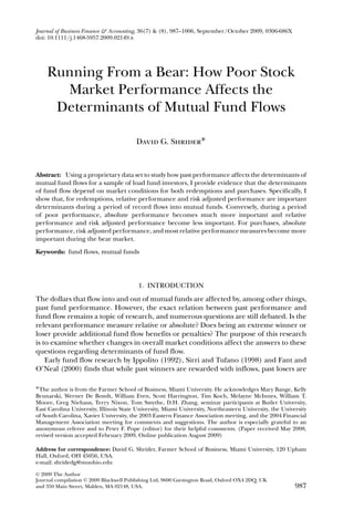
- 3. RUNNING FROM A BEAR 989 Figure 1 Standard & Poor’s 500-Stock Index versus Mutual Fund Flows Note: This figure graphs the level of the S&P 500 and total mutual fund inflows according to the 2006 Investment Company Fact Book from 1991–2002. During periods when the average fund flow changes, the determinants of fund flow are also more likely to change. Both redemption and purchase activity tend to be linked to past performance, and thus average fund flows are very different during my sample period when compared with earlier periods. Figure 1 shows similar trend lines for mutual fund inflows and the Standard & Poor’s 500-stock index from 1991 to 2002, which is the time period covered by O’Neal (2004) and Ivkovi´ and Weisbenner c (2007), as well as my data set. The Standard & Poor’s 500-stock index moves generally upward until 2000 when it begins a series of three down years. Overall flows into mutual funds suffer minor setbacks in 1994 and 1999, but the trend in fund flows generally follows stock market performance. Although flows generally follow the market, a lag is obvious: The market starts its decline in 2000, but inflows actually hit a high in 2001 before dropping sharply in 2002. Therefore, my sample provides data from a time period in which fund flows are very different in the two years. In addition to differences in the level of fund flows, differences in the way past performance affects redemption decisions in bull and bear markets can also prove insightful. Namely, both Odean (1998) and Grinblatt and Keloharju (2001) find evidence that individual investors are reluctant to sell poor-performing investments. Although neither study focuses on mutual fund trades, the suggestion that investors hold on to losers is consistent with the notion that poor-performing funds do not experience large outflows. Odean (1999), who examines the purchase behavior of no- load equity investors, finds that investors purchase stocks that have performed well in the past. Even though Odean’s sample does not include mutual fund trades, this result is consistent with the findings of the aggregate studies, namely, that mutual funds with good track records attract the bulk of mutual fund inflows. Although O’Neal (2004) finds that poor performers are punished, loss aversion is not an issue for mutual fund investors who measure gains and losses relative to their purchase price. That is, during bull markets, even the poorest performing funds, relative to a benchmark, see gains in absolute performance. C 2009 The Author Journal compilation C Blackwell Publishing Ltd. 2009
- 4. 990 SHRIDER While it is clear that past performance affects fund flow, the literature examines a host of other fund flow determinants. Del Guercio and Tkac (2001) and Faff et al. (2007) show that fund ratings affect flow. Kempf and Ruenzi (2008a) show that fund flows are related to the fund’s relative position within the fund family. Sirri and Tufano (1998) and Barber et al. (2002) show that fees and expenses are important determinants of fund flow. Other determinants include fund family structure (Massa, 2003), market volatility (Cao et al., 2008) and investor sentiment (Massa et al., 1999; and Indro, 2004). Before measuring differences by time period, I first show that my sample is representative of mutual funds in general by replicating findings in the prior literature and find that my results on overall fund flow are consistent with previous literature, including Ippolito (1992), Sirri and Tufano (1998) and Fant and O’Neal (2000). After controlling for raw performance, I find a large additional positive effect for the top performers but no additional negative effect for the worst performers. In other words, when only accounting for net flows, the punishment provided to the worst performers is not in sync with the reward given to the best performers. However, once I separate purchases and redemptions, my results based on the purchases of winners and the redemptions of losers are consistent with O’Neal (2004), Ivkovi´ and Weisbenner c (2007) and Cashman et al. (2006). Specifically, when I control for raw performance, I find no evidence that funds in the bottom decile see fewer redemptions. In fact, these funds experience redemption levels as large as would normally be expected, given their poor track record. While the stock market peaked in 2000, according to the Investment Company Institute (ICI, 2006), overall industry-wide fund flows did not hit a high until 2001 before experiencing a sharp decline in 2002. Therefore, to examine whether the determinants of fund flows are different between periods of good and poor performance, I measure redemption and purchase flows separately for 2001 and 2002. I find systematic differences when I test for the determinants of fund flows. First, consistent with Cashman et al. (2006), I find that during 2001, when net flows were still surging, relative return measures – such as the fund’s rank against other funds in the same Morningstar objective and rank in the top or bottom performance decile – are important in determining the percentage of redemptions. Second, consistent with Ivkovi´ and c Weisbenner (2007), I find that when testing the determinants of redemptions in 2002 when the fund performance was poor, the effect of absolute performance is nearly three times larger while the relative measures are much less important. The results for purchases show that whether past performance is measured by raw return, risk adjusted return, top-performing decile, or bottom-performing decile, investors are more affected by performance during the 2002 bear market. In sum, during a period in which new money is pouring into mutual funds, redemptions are sensitive to the fund’s rank against other funds in the same Morningstar objective (i.e., being one of the best or worst performers among all funds in the objective) and risk adjusted performance. In other words, under normal market conditions, when redeeming shares investors measure fund performance relative to other funds in the objective and relative to the level of risk the fund takes. However, when the market turns and investors begin to panic, absolute performance becomes much more important, trumping relative and risk adjusted performance measures. For purchases, investors become more discerning during a bear market as nearly all performance measures become more important. C 2009 The Author Journal compilation C Blackwell Publishing Ltd. 2009
- 5. RUNNING FROM A BEAR 991 This study contributes to the literature in two ways. First, it specifically addresses the open question in the literature of whether investors use relative or absolute performance when making redemption decisions. In fact, both relative and absolute measures of performance matter – but their importance differs depending on the market conditions faced by investors. Specifically, investors use relative performance in bull markets and absolute performance in bear markets when making redemption decisions while nearly all performance measures become more important when purchasing during a bear market. The second and broader contribution is that general market conditions affect investor behavior. While this is important in understanding mutual fund flows it is also important in any research involving individual investors. The remainder of the paper proceeds as follows. Section 2 discusses the data and method. Section 3 presents the results. Section 4 provides robustness checks, and Section 5 concludes. 2. DATA AND METHOD (i) Data The data are provided by a national full-service brokerage firm and include all mutual fund transactions during 2001 and 2002; a list of all funds in each account at year-end 2000, 2001 and 2002, for all accounts with at least one mutual fund holding; and the type of account. Panel A of Table 1 provides descriptive statistics for all accounts as of December 31, 2000. Of the total accounts, 39.6% are single or joint accounts; 13.3%, custodial; 38.9%, retirement; and 8.2%, other non-individual accounts. Based on value of holdings, 36.5% are single or joint accounts; 2.1%, custodial; 42.0%, retirement; and 19.1%, other non- individual accounts. On average, an account has 2.5 holdings, with the smaller custodial accounts averaging 1.6 holdings; single and joint accounts, 2.4 holdings; and retirement accounts, 3.0 holdings. New accounts are added to the data set throughout the sample period, and the transactions from the new accounts are included in the analysis. As shown in Table 1, Panel B, by year-end 2001, the number of accounts (dollars invested) increased by 21.2% (6.4%), but the distribution of accounts across account types is similar to that at year-end 2000. See Panel B for full descriptive statistics for accounts as of December 31, 2001. Table 2 provides descriptive information on the transactions within single and joint accounts, custodial accounts, retirement accounts, and other accounts between January 1, 2001 and December 31, 2002. Nearly one-fourth of all transactions are redemptions and more than three-fourths are purchases. The average size of redemptions and purchases are similar. The mean (median) redemption is $8,007 ($3,300) and the mean (median) purchase size is $9,612 ($4,749). (ii) Performance Measures To examine how investor transaction decisions are related to past performance, I conduct tests using past performance measures. Because Del Guercio and Tkac (2002), who compare pension fund and mutual fund investors, find that mutual fund investors base their decisions on raw return numbers rather than risk adjusted performance, I measure performance with raw one year total returns. Jain and Wu’s (2000) results C 2009 The Author Journal compilation C Blackwell Publishing Ltd. 2009
- 6. 992 Table 1 Account Characteristics Panel A: Account Characteristics as of December 31, 2000 % of Mean Median Std. Dev. Avg. No. Mean Median Std. Dev. of % of Total Total Acct. Acct. of Acct. MF of % of Holding Holding Holding Value of MF Type of Account Accounts Size ($) Size ($) Size ($) Holdings Value Size ($) Size ($) Size Holdings Single 20.0 35,947 11,558 82,458 2.4 19.4 15,041 7,580 26,621 19.4 Joint 19.6 32,285 12,095 73,925 2.3 17.1 13,821 7,242 25,061 17.2 Custodian 13.3 5,832 1,899 12,864 1.6 2.1 3,753 1,615 6,715 2.2 Trust 6.6 88,243 38,066 1,368,144 3.1 15.6 28,291 14,935 209,572 15.6 Partnership 0.1 157,372 42,279 388,435 3.4 0.4 46,295 20,331 86,491 0.4 Investment club 0.0 6,398 1,700 19,738 1.6 0.0 4,091 1,456 7,406 0.0 SHRIDER Corporation 0.5 98,011 27,978 343,091 2.7 1.3 36,324 15,029 97,866 1.3 Church 0.1 55,893 19,506 141,006 2.2 0.2 24,918 12,505 44,425 0.2 Bank 0.0 1,082,058 50,733 6,964,942 7.7 0.1 141,242 41,450 330,442 0.1 Estate 0.1 84,602 39,419 126,058 2.7 0.2 31,556 17,688 44,139 0.2 Regular IRA 27.5 51,610 22,771 89,796 3.3 38.4 15,716 8,791 22,925 38.4 SEP IRA 2.0 43,099 15,536 80,579 3.3 2.3 13,168 6,574 21,571 2.3 Journal compilation Roth IRA 7.1 5,448 2,049 17,842 1.9 1.0 2,857 1,303 6,906 1.1 C Simple IRA 2.3 5,492 2,805 7,146 2.0 0.3 2,729 1,416 3,822 0.3 Other 0.8 3.0 1.3 1.3 Total 100.0 2.5 100.0 100.0 Blackwell Publishing Ltd. 2009 C 2009 The Author
- 7. Table 1 (Continued) C 2009 The Author Journal compilation C Panel B: Account Characteristics as of December 31, 2001 % of Mean Median Std. Dev. Avg. No. Mean Median Std. Dev. of % of Total Total Acct. Acct. of Acct. MF of % of Holding Holding Holding Value of MF Type of Account Accounts Size ($) Size ($) Size ($) Holdings Value Size ($) Size ($) Size Holdings Single 18.9 32,563 10,049 75,625 2.5 19.0 13,149 6,166 24,449 19.0 Joint 18.1 29,297 10,561 67,796 2.4 16.3 12,064 5,876 22,698 16.3 Custodian 12.6 4,903 1,540 11,971 1.6 1.9 3,062 1,247 6,170 1.9 Trust 6.2 81,560 35,203 1,228,868 3.2 15.7 25,339 13,033 183,791 15.7 Partnership 0.1 149,133 36,347 368,935 3.5 0.4 42,467 17,849 87,004 0.4 Blackwell Publishing Ltd. 2009 Investment club 0.0 5,411 1,522 18,920 1.6 0.0 3,448 1,371 7,272 0.0 Corporation 0.5 93,014 24,864 349,886 2.7 1.3 33,900 12,854 107,946 1.3 Church 0.1 53,970 19,105 132,513 2.3 0.2 23,368 11,328 41,039 0.2 Bank 0.0 1,584,172 45,273 10,204,552 8.7 0.1 181,625 40,005 439,827 0.1 Estate 0.1 76,621 33,611 122,817 2.7 0.2 28,600 15,425 43,671 0.2 Regular IRA 28.6 44,974 19,179 80,139 3.4 39.6 13,195 6,965 20,257 39.6 RUNNING FROM A BEAR SEP IRA 2.0 36,163 12,422 71,072 3.4 2.3 10,657 4,944 18,916 2.3 Roth IRA 9.3 4,323 1,978 13,377 2.1 1.2 2,061 974 4,997 1.2 Simple IRA 2.7 5,665 3,003 7,186 2.3 0.5 2,511 1,328 3,522 0.5 Other 0.7 3.1 1.2 1.2 Total 100.0 2.7 100.0 100.0 Notes: This table provides the characteristics of accounts with mutual fund holdings from a national full-service brokerage firm. Panel A provides information from accounts at the beginning of the sample period, December 31, 2000 and Panel B provides the same data as of December 31, 2001. MF = mutual fund. 993
- 8. 994 SHRIDER Table 2 Transaction Data % Transactions Mean ($) Median ($) Std. Dev. ($) Panel A: Redemptions Trade size Full sample 23.8 8,007 3,300 19,515 Joint and single 8.0 7,864 3,505 17,459 Custodial 0.7 3,690 2,393 4,335 IRAs 12.5 7,116 3,001 14,217 Other 2.6 14,000 5,000 38,005 NAV 18.77 17.20 8.81 Panel B: Purchases Trade size Full sample 76.2 9,612 4,749 21,682 Joint and single 21.6 10,030 4,996 22,846 Custodial 1.7 3,974 2,454 5,101 IRAs 44.1 8,605 4,247 14,902 Other 8.8 15,331 6,887 40,913 NAV 20.38 18.40 9.13 Notes: This table provides data on transactions from all accounts for 2001 and 2002. Panel A (Panel B) provides data for redemptions (purchases). % Transactions is the percentage of total transactions included in the study. NAV is the net asset value at which trades took place. support the use of one-year returns. While I follow Del Guercio and Tkac (2002) and use raw returns as my measure of absolute performance, I also use risk adjusted returns as a control variable. I use alpha from a Carhart (1997) four-factor model as my measure of risk adjusted return. 4 Evidence also suggests that mutual fund investors base decisions on performance relative to other funds. For example, Capon et al. (1996) find that published performance rankings are investors’ most important source of information for making investment decisions. Therefore, I use two different measures of relative performance. First, I use performance rank relative to all funds in the same Morningstar objective. I rank funds into percentiles from zero (worst performer) to 100 (best performer). I also identify winners (i.e., funds in the top decile) and losers (i.e., funds in the bottom decile) among the funds that are included on the approved list of the firm that provided the data. I use these measures to test whether placement among the very best or very worst performing funds has an additional effect. (iii) Aggregating Individual Account Data Because the focus of this research is on the impact of fund flows, I aggregate all of the data to the mutual fund level. By using aggregating individual investor data rather than overall aggregate fund flows I am able to examine purchases and redemptions separately. This approach provides insight into whether the incentives that arise from 4 In tests not reported in the paper, I also use Jensen’s alpha from the capital asset pricing model (CAPM) as a measure of risk adjusted performance. The results using CAPM alpha are not qualitatively different from those using Carhart alpha, as reported in Tables 5–8. C 2009 The Author Journal compilation C Blackwell Publishing Ltd. 2009
- 9. RUNNING FROM A BEAR 995 Table 3 Holdings by Asset Class Equity (%) Fixed Income (%) Balanced (%) Panel A: 2000 Sample 83.2 6.7 10.1 Aggregate load funds 85.4 9.4 5.2 Aggregate no-load funds 84.1 12.6 3.2 Panel B: 2001 Sample 80.7 7.1 12.3 Aggregate load funds 82.5 10.7 6.7 Aggregate no-load funds 79.7 17.6 2.6 Notes: Panel A (Panel B) provide data for 2000 (2001). The first row of each panel gives the percentage of assets within the data set that is held in equity funds, fixed income funds, and balanced funds. The aggregate load and no-load rows list the percentage of assets invested in equity, fixed income, and balanced funds for all load and no-load funds listed in Morningstar. asymmetric fund flow are driven by purchase decisions, redemption decisions, or a combination of the two. However, data aggregated at the individual investor level may not be representative of all load fund investors. Therefore, to determine whether the investors in my sample are similar to investors in general, I compare the asset classes of the funds they own to the overall averages of all funds in Morningstar as reported in Table 3, Panel A. In 2000, of the total holdings in my sample, 83.2% are in equity funds, 6.7% are in fixed income funds, and 10.1% are invested in balanced funds. This distribution of assets is similar to the allocation of assets by investors in general. Of the funds included in Morningstar as of December 31, 2000, load fund investors have 85.4% of their assets in equity funds, 9.4% in fixed income funds, and 5.2% in balanced funds, whereas no-load fund investors have 84.1% in equity funds, 12.6% in fixed income, and 3.2% in balanced funds. Results for year-end 2001, as reported in Panel B, are similar. Differences between this sample and mutual fund investors at large in the percentage of assets invested in retirement accounts could also affect whether or not these results are representative. However, my sample is similar to mutual fund investors in general. At year-end 2000, 42% of the assets in the sample are invested in retirement accounts compared with 36% for all mutual funds according to the ICI Mutual Fund Fact Book. The same numbers for year-end 2001 are 44% and 34%. 5 3. RESULTS (i) Net Fund Flow To compare the compatibility of my sample of mutual fund transactions between January 1, 2001 and December 31, 2002 at national full-service broker-dealer 6 with 5 Another way to examine these data is to study the decision-making of individual investors, which is a topic of ongoing research. In that analysis, controlling for a fund being held in a retirement account does not qualitatively affect the other results. 6 I only omit trades of less than $1,000 and trades that could have been exchanges, but instead the same account made both a purchase and a redemption on the same day and paid a sales charge. These potential C 2009 The Author Journal compilation C Blackwell Publishing Ltd. 2009
- 10. 996 SHRIDER prior fund flow studies, I employ an OLS regression to examine the combined fund flow. The dependent variable used in the analysis is the proportion of fund flows to dollars in the fund. This fund flow proportion (FFP) for fund f during month t is defined as: f f DPt − DRt FFP f,t = f , (1) DHt where: f DPt = dollar value of shares purchased of fund f during month t; f DRt = dollar value of shares redeemed of fund f during month t; and f DHt = total dollar value of shares held of fund f at the beginning of month t. I use OLS regression on the following model: FFP f,t = α0 + β1 Return f,t + β2 Rank Obj f,t + β3 Winner f,t + β4 Loser f,t + β5 Alpha f,t + β6 B Share f,t + β7 C Share f,t + β7 Fixed Income f,t (2) + β7 Balanced f,t + β7 Expense Ratio f,t + β8 Log Total Value f,t + β9 Log TNA f,t + β10 Age f,t + 23 Month Dummies + ε f,t , f = 1, . . . , n, where Return f ,t is the one year total return for the year prior to time t; Rank Obj f ,t is the rank of the fund within its Morningstar objective over the year prior to time t; Winner f ,t is a binary variable, which equals 1 if fund f is in the top-performing decile ranked against other funds in the Morningstar objective for the year prior to time t, and zero otherwise; Loser f ,t is a binary variable, which equals 1 if fund f is in the bottom-performing decile ranked against other funds in the Morningstar objective for the year prior to time t, and zero otherwise; B Share f ,t is a dichotomous variable, which equals 1 if the fund t is a class B share, and zero otherwise; C Share f ,t is a dichotomous variable, which equals 1 if the fund t is a class C share, and zero otherwise; Alpha f ,t is a measure of risk adjusted performance that is the intercept from a regression of excess mutual fund returns on the four factors described in Carhart (1997); Expense Ratio f ,t is the expense ratio for fund f at time t; Log Total Value f ,t is the natural log of the total assets invested in the fund at the firm studied; Log TNA f ,t is the natural log of the total net assets for fund f at time t; and Age f ,t is the age in years of fund f at time t. There is some concern that collinearity is a problem as the return variables are correlated. Correlation coefficients of the return variables are shown in Table 4. Because the largest (in absolute value) correlation coefficient is −0.60, I run collinearity diagnostics. Condition indices show that collinearity is not a large problem as the largest condition indices are 24.18 and 12.97. In addition, I also run all models omitting each return variable individually. These results are qualitatively similar to those reported. The expected sign on Return, Rank Obj, Winner , and Alpha is positive because higher returns lead to more dollars invested in subsequent periods. Because prior research on exchanges might be the result of a conflict of interest between the client and the investment representative; however, as they only total 0.4% of all transactions, they do not skew the results. C 2009 The Author Journal compilation C Blackwell Publishing Ltd. 2009
- 11. RUNNING FROM A BEAR 997 Table 4 Correlation Coefficients Return Rank Obj. Winner Loser Alpha Return 1.00 Rank Obj 0.36 1.00 Winner 0.41 0.25 1.00 Loser −0.60 −0.30 −0.12 1.00 Alpha −0.15 0.21 0.06 0.12 1.00 Notes: This table presents correlation coefficients for the return variables. The return variables are the average annual total return over the past year (Return); the rank of the fund within its Morningstar objective (Rank Obj); a dichotomous variable, Winner (Loser ), which equals 1if the fund is in the top (bottom) performing decile of its Morningstar objective, and zero otherwise; the risk adjusted performance (Alpha) from a Carhart (1997) four-factor model. performance persistence (e.g., Brown and Goetzmann, 1995) suggests that the worst- performing funds are more likely to repeat as poor performers, one could expect the sign for Loser to be negative. However, Ippolito (1992), Sirri and Tufano (1998) and Fant and O’Neal (2000) all provide evidence that poor performers are not punished to the extent that winners are rewarded. The signs on B Share and C Share should be positive because investors avoid upfront sales charges. I expect the sign on Expense Ratio to be negative as investors try to avoid funds with higher fees. The signs for Log Total Value, Log TNA, and Age should all be positive as investors are more likely to buy funds that are popular at this particular firm as well as funds that are better known in general. The results, as reported in Table 5, are consistent with aggregate fund flow studies (Fant and O’Neal, 2000; Ippolito, 1992; and Sirri and Tufano, 1998) with respect to the sign and statistical significance of the coefficients for Return, Rank Obj, Winner , Loser and Alpha. I find that, on average, these funds experience larger purchases than redemptions. Past performance has a positive effect as the coefficient on Return is positive and statistically significant. The sign on the coefficients for the relative return measure, Rank Obj is also positive but not statistically significant. After controlling for general performance, being top decile of funds has an additional effect, which holds true across both time periods as the coefficient on Winner is positive and highly significant. The coefficient on Loser is negative as predicted, but it is not statistically significant. The coefficient on Alpha is positive and highly statistically significant. This finding that funds with positive risk adjusted performance attract additional flows is consistent with Jain and Wu (2000). The results for the control variables are generally consistent with the expected signs. More dollars flow into B and C shares as shown by the positive and statistically significant coefficients on the B Share and C Share variables. Both fixed income and balanced funds have larger fund flow proportions when compared to equity funds as the coefficients on Fixed Income and Balanced are both positive and statistically significant. Fewer dollars flow into funds with higher expense ratios as evidenced by the negative and statistically significant coefficient on the Exp Ratio variable. The positive and statistically significant sign on the coefficients of Log Total Value suggests that funds more widely held at the firm from which I obtained the data have larger fund flow proportions. However, after controlling for assets held at the firm, large funds and older funds have smaller fund C 2009 The Author Journal compilation C Blackwell Publishing Ltd. 2009
- 12. 998 SHRIDER Table 5 Fund Flows 1-Year FFP p-values Intercept 0.0477∗∗ 0.000 Return 0.0216∗∗ 0.000 Rank Obj 0.0013 0.407 Winner 0.0175∗∗ 0.000 Loser −0.0011 0.517 Alpha 0.0126∗∗ 0.000 B Share 0.0130∗∗ 0.000 C Share 0.0057∗∗ 0.000 Fixed Income 0.0055∗∗ 0.000 Balanced 0.0165∗∗ 0.000 Expense Ratio −0.0099∗∗ 0.000 Log Total Value 0.0034∗∗ 0.000 Log TNA −0.0050∗∗ 0.000 Age −0.0001∗ 0.011 Adj. R 2 0.0737 N 21,093 Notes: This table presents results from an ordinary least squares model on the fund flow proportion (FFP) as defined in equation (1). The independent variables are the average annual total return over the past year (Return); the rank of the fund within its Morningstar objective (Rank Obj); a dichotomous variable, Winner (Loser ), which equals 1 if the fund is in the top (bottom) performing decile of its Morningstar objective, and zero otherwise; the risk adjusted performance (Alpha) from a Carhart (1997) four-factor model; a dichotomous variable, (B Share (C Share)), which equals 1 if the fund is a B share (C share), and zero otherwise; a dichotomous variable (Fixed Income (Balanced)) if the fund is a fixed income (balanced) mutual fund; the expense ratio for the fund (Expense Ratio); the natural log of the total amount invested in a given fund at the broker-dealer that provided the data (Log Total Value); and the natural log of the total net assets of the fund (Log TNA); and the age of the fund in years (Age). Fixed time effects are included using month dummy variables. ∗∗ indicates statistical significance at the 0.01 level. ∗ indicates statistical significance at the 0.05 level. flow proportions, shown by the negative and statistically significant coefficients on Log TNA and Age. (ii) How Performance Affects Total Redemptions and Total Purchases I use the proportion of fund holdings redeemed or purchased measured in dollar value of shares as the dependent variable in a separate analysis of the determinants of purchases and redemptions. The proportion of the value of shares redeemed in fund f during month t is defined as: f DRt $R f,t = f , (3) DHt where: f DRt = dollar value of shares redeemed of fund f during month t, and f DHt = total dollar value of shares of fund f at the beginning of month t. C 2009 The Author Journal compilation C Blackwell Publishing Ltd. 2009
- 13. RUNNING FROM A BEAR 999 The proportion of the value of shares purchased ($P f ,t ) is defined similarly. The mean value for $R f ,t ($P f ,t ) is 0.01 (0.02), and the standard deviation is 0.03 (0.05). The tobit model is: $R f,t ($P f,t ) = α0 + β1 Return f,t + β2 Rank Obj f,t + β3 Winner f,t + β4 Loser f,t + β5 Alpha f,t + β6 B Share f,t + β7 C Share f,t + β7 Fixed Income f,t (4) + β7 Balanced f,t + β7 Expense Ratio f,t + β8 Log Total Value f,t + β9 Log TNA f,t + β10 Age f,t + 23 Month Dummies + ε f,t , f = 1, . . . , n. The coefficients reported in Table 6 represent the marginal effect of a one-unit change in the explanatory variable on the expected value of the proportion of the fund that is purchased or redeemed in a given month. For the dichotomous variables such as Winner and Loser , the marginal effects are calculated by changing the variable from zero to 1. Marginal effects for all other variables are evaluated at the sample mean. The expected sign on Return, Rank Obj, Winner and Alpha is negative for redemptions and positive for purchases because higher returns should lead to fewer redemptions and more purchases in subsequent periods. The expected sign on Loser is the reverse – that is, positive for the redemption specifications and negative for the purchase specifications. Because buy-and-hold investors self-select into A shares and because A shares have higher initial costs in the form of the upfront sales charge, I expect the sign on the alternatives B Share and C Share to be positive for both purchases and redemptions. Expense Ratio should have a positive sign for redemptions and a negative sign for purchases as investors try to avoid funds with higher fees. Finally, Log Total Value, Log TNA and Age should all have negative signs for redemptions and positive signs for purchases as investors are more likely to buy funds that are popular at the firm under study as well as funds that are better known in general. Tobit results for redemptions are found in the first column of Table 6. The results show that funds see more dollars redeemed when their performance is worse. This result is consistent with the expected result. The coefficient on the absolute performance variable, Return, is negative and statistically significant at the 1% level. The sign on the coefficients of the relative performance variable, Rank Obj, is also negative but not statistically significant. I include the Winner and Loser dummy variables to test whether an effect is associated with being an extreme performer. After controlling for total return, the results suggest that these investors sell larger proportions of the top-performing funds. The sign of the coefficient on Winner is positive and statistically significant at the 1% level. In other words, after controlling for performance, the best performers experience larger total redemptions than other funds. Although this result is counterintuitive, it is consistent with the results of Cashman et al. (2006) before they directly control for the persistence of fund flows. 7 The sign of the coefficient on Loser is positive, but not statistically significant. The sign on the coefficient on Alpha is positive and statistically significant. The last column of Table 6 shows the tobit results for purchases. The results for the Return variable are consistent with expected sign as the coefficient is positive and 7 Cashman et al. (2006) control for persistent fund flows by including a lagged fund flow term. I do not use this control in Table 6 in order to match the existing literature. However, I do control for persistent fund flows, in the same way as Cashman et al., in robustness checks by using the lagged dependent variable. C 2009 The Author Journal compilation C Blackwell Publishing Ltd. 2009
- 14. 1000 SHRIDER Table 6 Tobit Results Redemptions Purchases 1-Year 1-Year Return −0.0155∗∗ 0.0148∗∗ (0.000) (0.000) Rank Obj −0.0006 −0.0015 (0.394) (0.056) Winner 0.0043∗∗ 0.0134∗∗ (0.000) (0.000) Loser 0.0010 −0.0008 (0.123) (0.463) Alpha 0.0025∗∗ 0.0104∗∗ (0.000) (0.000) B Share 0.0036∗∗ 0.0130∗∗ (0.000) (0.000) C Share 0.0026∗∗ 0.0103∗∗ (0.000) (0.000) Fixed Income −0.0001 0.0016∗ (0.874) (0.017) Balanced 0.0001 0.0069∗∗ (0.881) (0.000) Expense Ratio 0.0007 −0.0091∗∗ (0.089) (0.000) Log Total Value 0.0018∗∗ 0.0061∗∗ (0.000) (0.000) Log TNA −0.0004∗∗ −0.0051∗∗ (0.002) (0.000) Fund Age −0.0001∗∗ −0.0001∗∗ (0.002) (0.048) N 20,985 20,976 Notes: This table presents results from a tobit model on the proportion of the fund redeemed or purchased in terms of dollars as defined in equation (3). The independent variables are the average annual total return over the past year (Return); the rank of the fund within its Morningstar objective (Rank Obj); a dichotomous variable, Winner (Loser ), which equals 1 if the fund is in the top (bottom) performing decile of its Morningstar objective, and zero otherwise; the risk adjusted performance (Alpha) from a Carhart (1997) four-factor model; a dichotomous variable (B Share (C Share)), which equals 1 if the fund is a B share (C share), and zero otherwise; a dichotomous variable (Fixed Income (Balanced)) if the fund is a fixed income (balanced) mutual fund; the expense ratio for the fund (Expense Ratio); the natural log of the total amount invested in a given fund at the broker-dealer that provided the data (Log Total Value); and the natural log of the total net assets of the fund (Log TNA); and the age of the fund in years (Age). Fixed time effects are included using month dummy variables. p-values are in parentheses. ∗∗ indicates statistical significance at the 0.01 level. ∗ indicates statistical significance at the 0.05 level. statistically significant at the 1% significance level. The sign on the Rank Obj variable is negative but not statistically significant. The sign on the coefficient on Alpha is positive and highly significant. These results indicate that more total purchases are made for funds that have high absolute performance and high risk adjusted performance. Even after controlling for performance, the sign of the coefficient on the Winner variable is positive and statistically significant at the 1% significance level. This finding suggests that while funds with better performance are rewarded with greater purchases, top C 2009 The Author Journal compilation C Blackwell Publishing Ltd. 2009
- 15. RUNNING FROM A BEAR 1001 performers are rewarded at an even greater rate than other funds. The coefficient on Loser is negative but not statistically significant. (iii) Test of Time Period Having established that the results of my sample are consistent with the existing literature’s understanding of aggregate fund flows and of the determinants of fund flow when purchases and redemptions are separated, I now focus on whether the determinants of fund flow change based on market conditions. To this end, I run separate tobit models on equation (4) for 2001 and 2002. As shown in Figure 1, mutual funds in general saw record inflows in 2001 before fund flows declined precipitously in 2002. The expected signs for the results of redemptions (purchases) in Table 7 (Table 8) are the same as those discussed previously for the redemptions and purchases in Table 6. Like Table 6, the coefficients in Tables 7 and 8 represent marginal effects. The results for redemptions by year are reported in Table 7. The first column reports the results for 2001 and the second column shows the results for 2002. The coefficient on Return, which is simply the absolute performance, is negative and statistically significant in both the 2001 and 2002 specifications. However, the size of the coefficient is nearly three times larger in the 2002 bear market specification. A pattern can be seen in the results for the three relative performance measures, Rank Obj, Winner and Loser : That is, relative performance is more important in 2001 than in 2002. All of the coefficients are statistically significant at nearly the 1% significance level in 2001. In the bear market specification neither Rank Obj nor Loser are statistically significant and the size of the coefficient on Winner is smaller than in the 2001 specification. The same pattern holds for Alpha, the measure of risk adjusted fund performance. Alpha is significant at the 1% significance level in 2001, but it is not statistically significant in 2002. These results are consistent with the idea that investors spend more time combing through numbers when markets are normal, but in a bear market, they are focused on exiting funds and primarily concerned with absolute performance. C Share and Expense Ratio exhibit a similar pattern and support the idea that investors focus on absolute performance in bear markets. The coefficient on C Share is positive and statistically significant at better than the 1% significance level in the normal market (2001) specification but it is not statistically significant in the bear market (2002) specification. This finding is consistent with the notion that in a normal market, investors are more willing to redeem C shares when compared with A shares for which they paid an upfront sales charge, but in a bear market, the loss of this sunk cost is no longer a high priority and the difference between C shares and A shares becomes insignificant. The coefficient on Expense Ratio is statistically significant in both specifications, but the sign changes from negative in the 2001 specification to positive in the 2002 specification. These results indicate that funds with higher expense ratios actually see fewer redemptions in normal markets, but in bear market conditions, funds that take more expenses out of their returns see more redemptions. The results on B Share are virtually identical between 2001 and 2002. Fixed income funds are more likely to see redemptions in 2002 while balanced funds are less likely. The results on Log Total Value, Log TNA and Age are inconsistent across specifications and often counter to their expected signs. Taken together, these results suggest that these variables do not substantially control fund reputation among investors. C 2009 The Author Journal compilation C Blackwell Publishing Ltd. 2009
- 16. 1002 SHRIDER Table 7 Tobit Results by Year: Redemptions 1-Year 2001 2002 Return −0.0125∗∗ −0.0322∗∗ (0.000) (0.000) Rank Obj −0.0023∗∗ 0.0004 (0.006) (0.695) Winner 0.0056∗∗ 0.0051∗∗ (0.000) (0.000) Loser −0.0019∗ 0.0001 (0.019) (0.902) Alpha 0.0039∗∗ 0.0010 (0.000) (0.082) B Share 0.0035∗∗ 0.0038∗∗ (0.000) (0.000) C Share 0.0058∗∗ −0.0007 (0.000) (0.356) Fixed Income 0.0007 0.0021∗∗ (0.224) (0.005) Balanced 0.0030∗∗ 0.0001 (0.002) (0.943) Expense Ratio −0.0025∗∗ 0.0042∗∗ (0.000) (0.000) Log Total Value 0.0025∗∗ 0.0011∗∗ (0.000) (0.000) Log TNA −0.0024∗∗ 0.0017∗∗ (0.000) (0.000) Age 0.0000 −0.0001∗∗ (0.488) (0.000) N 9,787 11,198 Notes: This table presents results from a tobit model on the proportion of the fund redeemed or purchased in terms of dollars as defined in equation (3). The independent variables are the average annual total return over the past year (Return); the rank of the fund within its Morningstar objective (Rank Obj); a dichotomous variable, Winner (Loser ), which equals 1 if the fund is in the top (bottom) performing decile of its Morningstar objective, and zero otherwise; the risk adjusted performance (Alpha) from a Carhart (1997) four-factor model; a dichotomous variable (B Share (C Share)), which equals 1 if the fund is a B share (C share), and zero otherwise; a dichotomous variable (Fixed Income (Balanced)) if the fund is a fixed income (balanced) mutual fund; the expense ratio for the fund (Expense Ratio); the natural log of the total amount invested in a given fund at the broker-dealer that provided the data (Log Total Value); and the natural log of the total net assets of the fund (Log TNA); and the age of the fund in years (Age). Fixed time effects are included using month dummy variables. p-values are in parentheses. ∗∗ indicates statistical significance at the 0.01 level. ∗ indicates statistical significance at the 0.05 level. The purchase results, reported in Table 8, also show a difference between 2001 and 2002. However, the difference is not between absolute and relative performance as is the case with the redemptions. In the 2001 period, investors purchased past winners and funds with positive risk adjusted performance as shown by the positive and significant coefficients on Winner and Alpha while the coefficients on Return and Loser are statistically insignificant and the coefficient on Rank Obj is negative. However, the bear market specification shows that investors became very concerned about all returns C 2009 The Author Journal compilation C Blackwell Publishing Ltd. 2009
- 17. RUNNING FROM A BEAR 1003 Table 8 Tobit Results by Year: Purchases 1-Year 2001 2002 Return 0.0032 0.0620∗∗ (0.213) (0.000) Rank Obj −0.0037∗∗ 0.0003 (0.003) (0.832) Winner 0.0088∗∗ 0.0141∗∗ (0.000) (0.000) Loser −0.0004 0.0042∗ (0.775) (0.016) Alpha 0.0077∗∗ 0.0106∗∗ (0.000) (0.000) B Share 0.0088∗∗ 0.0158∗∗ (0.000) (0.000) C Share 0.0124∗∗ 0.0078∗∗ (0.000) (0.000) Fixed Income −0.0006 0.0021 (0.484) (0.051) Balanced 0.0060∗∗ 0.0069∗∗ (0.000) (0.000) Expense Ratio −0.0065∗∗ −0.0093∗∗ (0.000) (0.000) Log Total Value 0.0048∗∗ 0.0074∗∗ (0.000) (0.000) Log TNA −0.0048∗∗ −0.0048∗∗ (0.000) (0.000) Age 0.0000 −0.0003∗∗ (0.851) (0.000) N 9,786 11,190 Notes: This table presents results from a tobit model on the proportion of the fund redeemed or purchased in terms of dollars as defined in equation (3). The independent variables are the average annual total return over the past year (Return); the rank of the fund within its Morningstar objective (Rank Obj); a dichotomous variable, Winner (Loser ), which equals 1 if the fund is in the top (bottom) performing decile of its Morningstar objective, and zero otherwise; the risk adjusted performance (Alpha) from a Carhart (1997) four-factor model; a dichotomous variable (B Share (C Share)), which equals 1 if the fund is a B share (C share), and zero otherwise; a dichotomous variable (Fixed Income (Balanced)) if the fund is a fixed income (balanced) mutual fund; the expense ratio for the fund (Expense Ratio); the natural log of the total amount invested in a given fund at the broker-dealer that provided the data (Log Total Value); and the natural log of the total net assets of the fund (Log TNA); and the age of the fund in years (Age). Fixed time effects are included using month dummy variables. p-values are in parentheses. ∗∗ indicates statistical significance at the 0.01 level. ∗ indicates statistical significance at the 0.05 level. when making purchases in 2002. Specifically, the coefficients on Return, Winner and Alpha, are all statistically significant at the 1% significance level, while Loser is significant at the 5% level. The positive sign on Loser indicates that the worst performers see larger purchases than would be predicted by their return. The signs on the control variables are somewhat consistent with expectations in the purchase specifications found in Table 8. B Share, C Share, Expense Ratio and Log Total C 2009 The Author Journal compilation C Blackwell Publishing Ltd. 2009
- 18. 1004 SHRIDER Value are consistent with the expected sign in both specifications. Fixed Income is not significant in either year while Balanced is positive and statistically significant at the 1% level in both years. As in the previous findings, Log TNA and Age are not consistent with the expected sign across both specifications. While the results between redemptions and purchases are not the same, they are both consistent with the idea that investors are reacting to a bear market. When making redemptions under normal conditions, relative performance measures and risk adjusted performance are the most important factors in terms of fund flows. But, in the bear market of 2002 raw returns become the most important factor of fund flows as investors rapidly exit funds. For purchases, investors become very selective as raw return, risk adjusted return, and most relative performance measures become more important when selecting funds to purchase during the 2002 bear market period. 4. ROBUSTNESS Because the main focus of this study is whether the determinants of fund flow differ in good and bad markets, the definitions of a good market and bad market are very important. The beginning of the market correction could be marked by, among other things, the Dow Jones Industrial Average’s high on May 22, 2001, the unexpected shock of September 11, 2001, or the peak in fund flows late in 2001; therefore, I conduct tests in which I divide my time period at different points before and after year-end 2001. The results (not tabulated) are not significantly different from those reported in Tables 7 and 8. Robustness results show the same general pattern when the split is close to the calendar-year split reported here and becomes progressively weaker the further the split moves (in either direction) from year-end 2001. Cashman et al. (2006) show that fund flows are very persistent and that controlling for this persistence with the lagged dependent variable causes the results to better match expected signs. When the lagged dependent variable is included, the sign on the lagged dependent variable is positive and highly statistically significant in all specifications, however, none of the other results are qualitatively changed. To test further for robustness, I model all of the tobit specifications using a two-step process based on (a) whether to make a transaction and (b) the size of the transaction, using a Heckman (1979) procedure. The results (not tabulated) using this process are qualitatively similar to the tobit model results. None of the inverse mills ratios from the first step (probit) are statistically significant at the 5% level in the second step (OLS). I also run robustness checks on the size variables. Because Log Total Value and Log TNA are positively correlated (correlation coefficient = 0.69) and because they have the largest variance inflation factors, I run all tests without Log Total Value. I find that dropping Log Total Value does not cause the results to be qualitatively different from those previously reported. 5. CONCLUSION This paper investigates whether the determinants of fund flow are affected by the shifting market conditions by examining the performance of a sample of mutual funds during 2000 (strong fund flow market) and 2001 (weak fund flow market). To determine whether my sample and, thus, my findings are comparable to previous literature, I first replicate the results of the prior studies. Specifically, my results for C 2009 The Author Journal compilation C Blackwell Publishing Ltd. 2009
- 19. RUNNING FROM A BEAR 1005 aggregate fund flows show that winners are rewarded to a greater degree than losers are punished, which is consistent with Ippolito (1992), Sirri and Tufano (1998) and Fant and O’Neal (2000). When I separate purchases and redemptions, I find evidence that losers see large redemptions but that these redemptions are masked by new purchases, which is consistent with O’Neal (2004), Ivkovi´ and Weisbenner (2007) and Cashman c et al. (2006). After I establish that my study sample is, in fact, in line with previous research, I address whether the determinants of mutual fund flows are affected by market conditions. I find that redemptions are strongly affected by relative performance and risk adjusted performance under normal market conditions. However, in bear market conditions, redemptions are more strongly affected by absolute performance, and measures of relative performance and risk adjusted performance become less important. For purchases, absolute performance, risk adjusted performance, and most relative performance measures become more important in 2002 than in 2001. This study contributes to the literature in both a specific and a general way. First, it provides evidence that mutual fund flows are affected by relative, risk adjusted and absolute performance measures. However, which performance measures are the most relevant depends on overall market conditions. In a more general way this study shows the importance of including controls for market conditions in future individual investor research. REFERENCES Acker, D. and N. Duck (2006), ‘A Tournament Model of Fund Management’, Journal of Business Finance & Accounting , Vol. 33, pp. 1460–83. Barber, B., T. Odean and L. Zheng (2002), ‘Out of Sight, Out of Mind: The Effects of Expenses on Mutual Fund Flows’, Journal of Business, Vol. 78, pp. 2095–119. Brown, K., W. Harlow and L. Starks (1996), ‘Of Tournaments and Temptations: An Analysis of Managerial Incentives in the Mutual Fund Industry’, The Journal of Finance, Vol. 51, pp. 85–110. Brown, S. and W. Goetzmann (1995), ‘Performance Persistence’, Journal of Finance, Vol. 50, pp. 679–98. Cao, C., E. Chang and Y. Wang (2008), ‘An Empirical Analysis of the Dynamic Relationship Between Mutual Fund Flow and Market Return Volatility’, Journal of Banking and Finance, Vol. 32, pp. 2111–23. Capon, N., G. Fitzsimmons and R. Prince (1996), ‘An Individual Level Analysis of the Mutual Fund Investment Decision’, Journal of Financial Services Research, Vol. 10, pp. 59–82. Carhart, M. (1997), ‘On Persistence in Mutual Fund Performance’, The Journal of Finance, Vol. 52, pp. 57–82. Cashman, G., D. Deli, F. Nardari and S. Villupuram (2006), ‘Investors Do Respond to Poor Mutual Fund Performance: Evidence from Inflows and Outflows’, Working Paper (Arizona State University). Chevalier, J. and G. Ellison (1997), ‘Risk Taking by Mutual Funds as a Response to Incentives’, Journal of Political Economy, Vol. 105, pp. 1167–200. Del Guercio, D. and P. Tkac (2001), ‘Star Power: The Effect of Morningstar Ratings on Mutual Fund Flows’, Working Paper (Federal Reserve Bank of Atlanta). ——— ——— (2002), ‘The Determinants of the Flow of Funds of Managed Portfolios: Mutual Funds versus Pension Funds’, Journal of Financial and Quantitative Analysis, Vol. 37, pp. 523–57. Edelen, R. and J. Warner (2001), ‘Aggregate Price Effects of Institutional Trading: A Study of Mutual Fund Flow and Market Returns’, Journal of Financial Economics, Vol. 59, pp. 195–220. C 2009 The Author Journal compilation C Blackwell Publishing Ltd. 2009
- 20. 1006 SHRIDER Faff, R., J. Parwada and H. Poh (2007), ‘The Information Content of Australian Managed Fund Ratings’, Journal of Business Finance & Accounting , Vol. 34, pp. 1528–47. Fant, L. F. and E. O’Neal (2000), ‘Temporal Changes in the Determinants of Mutual Fund Flows’, Journal of Financial Research, Vol. 23, pp. 353–72. Goetzmann, W. and N. Peles (1997), ‘Cognitive Dissonance and Mutual Fund Investors’, Journal of Financial Research, Vol. 20, pp. 145–58. Grinblatt, M. and M. Keloharju (2001), ‘What Makes Investors Trade?’, Journal of Finance, Vol. 56, pp. 589–616. ——— and S. Titman (1992), ‘The Persistence of Mutual Fund Performance’, The Journal of Finance, Vol. 47, pp. 1977–84. ——— ——— (1993), ‘Performance Measurement Without Benchmarks: An Examination of Mutual Fund Returns’, Journal of Business, Vol. 66, pp. 47–68. Gruber, M. (1996), ‘Another Puzzle: The Growth in Actively Managed Mutual Funds’, The Journal of Finance, Vol. 51, pp. 783–810. Heckman, J. (1979), ‘Sample Selection Bias as a Specification Error’, Econometrica, Vol. 47, pp. 153–61. Hendricks, D., J. Patel and R. Zeckhauser (1993), ‘Hot Hands in Mutual Funds: Short-run Persistence of Relative Performance’, 1974-1988. The Journal of Finance, Vol. 48, pp. 93– 130. Indro, D. (2004), ‘Does Mutual Fund Flow Reflect Investor Sentiment?’ Journal of Behavioral Finance, Vol. 5, pp. 105–15. Investment Company Institute (2006), 2006 Investment Company Fact Book. Ippolito, R. (1992), ‘Consumer Reaction to Measures of Poor Quality: Evidence from the Mutual Fund Industry’, Journal of Law and Economics, Vol. 35, pp. 45–70. Ivkovi´ , Z. and S. Weisbenner (2007), ‘“Old” Money Matters: The Sensitivity of Mutual Fund c Redemption Decisions to Past Performance’, Working Paper (University of Illinois at Urbana-Champaign). Jain, P. and J. Wu (2000), ‘Truth in Mutual Fund Advertising: Evidence on Future Performance and Fund Flows’, Journal of Finance, Vol. 55, pp. 937–58. Johnson, W. (2007), ‘Who Monitors the Mutual Fund Manager, New or Old Shareholders?’ Working Paper (AFA 2006 Boston Meetings Paper). Kempf, A. and S. Ruenzi (2008a), ‘Family Matters: The Performance Flow Relationship in the Mutual Fund Industry’, Journal of Business Finance & Accounting , Vol. 35, pp. 77–99. ——— ——— (2008b), ‘Tournaments in Mutual-Fund Families’, Review of Financial Studies, Vol. 21, pp. 1013–36. Massa, M. (2003), ‘How Do Family Strategies Affect Fund Performance? When Performance- Maximization is Not the Only Game in Town’, Journal of Financial Economics, Vol. 67, pp. 249–304. ——— and R. Patgiri (2007), ‘Incentives and Mutual Fund Performance: Higher Performance or Just Higher Risk Taking?’ Working Paper (SSRN). ———, W. Goetzmann and K. Rouwenhorst (1999), ‘Behavioral Factors in Mutual Fund Flows’, Working Paper (Yale). Odean, T. (1998), ‘Are Investors Reluctant to Realize Losses?’ Journal of Finance, Vol. 53, pp. 1775–98. ——— (1999), ‘Do Investors Trade Too Much?’ American Economic Review, Vol. 89, pp. 1279–98. O’Neal, E. (2004), ‘Purchase and Redemption Patterns of US Equity Mutual Funds’, Financial Management, Vol. 33, pp. 63–90. Otten, R. and D. Bams (2002), ‘European Mutual Fund Performance’, European Financial Management, Vol. 8, pp. 75–101. Patel, J., R. Zeckhauser and D. Hendricks (1991), ‘The Rationality Struggle: Illustrations from Financial Markets’, American Economic Review, Vol. 81, pp. 232–36. Sirri, E. and P. Tufano (1998), ‘Costly Search and Mutual Fund Flows’, Journal of Finance, Vol. 53, pp. 1589–622. Wermers, R. (2003), ‘Is Money Really ‘Smart’? New Evidence on the Relation Between Mutual Fund Flows, Manager Behavior, and Performance Persistence’, Working Paper (SSRN). Zheng, L. (1999), ‘Is Money Smart? A Study of Fund Investors’ Fund Selection Ability’, Journal of Finance, Vol. 54, pp. 901–33. C 2009 The Author Journal compilation C Blackwell Publishing Ltd. 2009