This slideshow explains the factors that determine the trajectory of the federal debt and deficit over time. Perfect plug-in for online econ courses.

1. Is the Federal Budget
Out of Control?
A Tutorial on Debt Dynamics
and Sustainability
Ed Dolan
Senior Fellow, Niskanen Center
Revised March 2020
Terms of Use: These slides are provided under Creative Commons License Attribution—Share Alike 3.0 .

2. Out of Control?
 Even before the coronavirus crisis of 2020, many people feared that the federal
budget was out of control.
 Are fears of an exploding debt and deficit realistic?
 This tutorial explains the dynamics of the debt and deficit and the conditions
needed for fiscal sustainability.
CBO

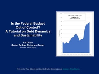
3. How to Measure the Debt
 Debt held by the public, also known
as net debt, is the best measure of
federal borrowing.
 The debt ratio is the ratio of net debt
to GDP, 79.2% as of 2019.
 About 40% of net debt was owned by
foreign investors.
 Gross debt includes debt owed by
one government agency to another – a
bookkeeping entry that puts no net
burden on the economy. As of 2019
gross debt was about 107% of GDP.
US federal debt, 2019:
• Net debt = $13.8 trillion
• Debt ratio (net debt/GDP) = 79.2%
Data source: Congressional Budget Office

4. Debt vs. Deficit
 The government debt is the total
amount that the government
owes.
 The budget balance is equal to
government revenues minus
expenditures, a negative number
when there is a deficit and a
positive number when there is a
surplus.
 Each year the debt changes by
the amount of the budget
balance.

5. Adjusting for the Business Cycle
 To identify long-run debt trends,
we need adjust for the effects of
the business cycle.
 Key terms:
 Potential GDP is an estimate of the
total output that the economy could
produce in the long-run without
overheating the economy, popularly
known as “full employment GDP.”
 The output gap is equal to current
GDP minus potential GDP, usually
stated as a percent of potential
GDP.
 The output gap is negative at the
trough of the cycle and positive at
the peak.

6. Automatic Stabilizers
 Automatic stabilizers are line items
that automatically move the budget
balance toward deficit when the output
gap is negative and toward surplus
when it is positive, even if there are no
changes in tax or spending laws.
 Examples:
 Income tax revenues increase when the
economy expands, pushing the balance
toward surplus.
 Unemployment benefits increase when the
economy is in recession, pushing the
balance toward deficit.

7. Current vs. Structural Budget Balance
 The current balance of the budget is
each year’s measured value of
revenues minus expenditures.
 The structural balance (sometimes
called the cyclically adjusted
balance) is the current balance minus
the contribution of automatic stabilizers.
 The structural balance shows what the
budget balance would be under current
laws in force if the output gap were
zero.

8. The Primary Structural Balance
 The primary structural balance (PSB)
is equal to the overall structural balance
excluding interest payments on the
government debt.
 Interest on the debt is excluded because it
depends on decisions made in the past, not
on current policy.
 Expenditures excluding interest are called
program expenditures.
 The PSB is a key determinant of long-
run debt trends.
Example 1 (all numbers are
percent of potential GDP):
• Structural balance = -5%
• Interest payments = 2%
• Primary structural balance =
-3%
• Both the primary structural
balance and overall structural
balance are in deficit
Example 2:
• Structural balance = -1.5%
• Interest payments = 2%
• PSB = +0.5%
• The overall structural balance
is in deficit but the PSB is in
surplus

9. US Budget Balances, 1970-2019
 This figure shows three US
government budget balances for
1970-2019.
 In a recession year (e.g. 2009)
the current balance is below the
structural balance (larger deficit).
 Near the peak of the cycle the
current balance is above the
structural balance (smaller deficit,
as in 1979, or larger surplus, as
in 2000).
 The primary structural balance is
always above the current
structural balance by a distance
equal to interest on the debt.

10. The Steady-State Primary Structural Balance
 Under any given conditions, there is
some primary structural balance just
sufficient to hold total government debt
constant as a share of GDP.
 We will call that the steady-state value
of the PSB, or PSB*.
 The panel at the right shows how to
calculate PSB* given the debt ratio, the
interest rate on the debt, and the rate of
growth of GDP.
Let . . .
• PSB* = the steady-state
value of the primary structural
balance
• DEBT = the initial ratio of
debt to GDP
• INT = Interest rate on
government debt
• GRO = Rate of growth of
GDP
Then . . .
PSB* = DEBT(INT-GRO)
Note: The interest rate and growth rate can
be stated in either nominal or real terms,
provided both are stated the same way

11. Example 1:
 DEBT = 0.5
 INT = 0.02
 GRO = 0.04
 PSB* = 0.5(0.02-0.04) = -0.01
Example 1: The Math
 If there is a constant primary structural
balance of -1% of GDP (a deficit), the
debt ratio will be constant at 50% of
GDP.
 If PSB <-1% (a greater deficit) the debt
will grow.
 If PSB>-1% (a smaller deficit or a surplus)
the debt will shrink.
 Total interest payments (INT times
DEBT) will be 1% of GDP, so stability
of the debt implies an initial overall
structural balance of -2% (a structural
deficit).

12. Example 1: Dynamics
 In Example 1, the interest rate
(0.02) is less than the rate of GDP
growth (0.04)
 If the PSB is lower than PSB* (e.g.
―0.015 instead of the steady state
value of ―0.01), the debt ratio will
grow toward a new steady-state
value, in this case 0.75
 If the PSB is larger than PSB* (e.g.
― .005), the debt ratio will
decrease toward a new steady-
state value, in this case 0.25
PSB= -.015
PSB*= -.01
PSB= -.005
Dynamics of Debt as % of GDP
DEBT=0.5 INT=0.02 GRO=0.04

13. Example 2
 DEBT = 0.5
 INT = 0.04
 GRO = 0.02
 PSB* = 0.5(0.04-0.02) = +0.01
Example 2: The Math
 If there is a constant primary
structural surplus of 1% of GDP, the
debt ratio will remain constant at
50% of GDP
 If PSB <1% (a smaller surplus or a
deficit) the debt will grow.
 If PSB>1% the debt will shrink.
 Total interest payments (INT times
DEBT) will be 2% of GDP, so
stability of the debt requres an initial
overall structural balance, including
interest of -1% (a structural deficit).

14. Example 2: Dynamics
 In Example 2, the interest rate (0.04)
is greater than the rate of GDP
growth (0.02).
 If the PSB is less than the steady-
state value of 0.01 (e.g. 0.005) the
debt ratio will grow without limit at an
ever increasing rate.
 If the PSB is greater than the steady
state value (e.g. 0.015), the debt
ratio will decrease without limit.
 A negative net debt ratio means the
government has financial assets that
exceed its financial liabilities, as in
Norway and some other oil-rich
countries.
PSB=.005
PSB*=.01
PSB=.015
Dynamics of Debt as % of GDP
DEBT=0.5 INT=0.04 GRO=0.02

15. Interest vs. Growth Rates: Why it Matters
 The debt will “explode,” that is,
grow without limit at an ever faster
rate, only if the rate of interest is
higher than the rate of growth of
potential GDP.
 If interest rates are lower than
growth rates, the debt ratio will
have a finite ceiling.
 Shown in chart:
 Net interest paid/net debt (the
average rate on outstanding debt.)
 5-year moving geometric average of
growth of potential nominal GDP.
 10-year Treasury rate (an
approximation of the cost of issuing
new debt.)

16. Interest vs. Growth Rates in the Inflationary 60s and 70s
 The 1960s and 1970s were a
period of rapid GDP growth and
constantly accelerating inflation.
 Nominal interest rates were low
relative to nominal GDP growth
during those years, probably in part
because bond buyers chronically
underestimated future inflation.

17. Interest vs. Growth Rates: The 1980s and 1990s
 In the 1980s and 1990s, inflation
slowed steadily.
 Nominal interest rates averaged
higher than the growth of nominal
potential GDP in those years,
probably because bond buyers
overestimated the risk that high
inflation would return. (It did not.)

18. Lower Interest Rates Appear to be the New Normal
 Since 2000, interest rates have
been low and potential nominal
GDP has grown a moderate rate of
averaging about 4 percent.
 During this period, interest rates
have averaged below the growth of
GDP, a situation that has come to
be seen as the new normal.
 Interest rates lower than GDP
growth imply low risk of an
“exploding” debt.

19. 2017 to 2019: An Unusual Pattern of Fiscal Policy
 Fiscal policy in the years 2017-2019
had an unusual procyclical pattern.
 Due in part to large tax cuts and in
part to higher spending, the PSB
moved sharply toward deficit just as
the output gap closed and then
became positive.
 That contrasted with the
countercyclical pattern of fiscal policy
for most of the preceding 50 years,
under which the PSB moved toward
surplus during the approach to
cyclical peaks.

20. The Situation as of 2019
 As of 2019, debt was about 80% of
GDP, interest expenditures were
about 2.3 percent of the debt, and
the growth of nominal GDP was
about 4%.
 A primary structural balance of -1.36
would have been required to hold
the debt ratio constant at 80%.
 Instead, the actual PSB was 2.9%.
With no change in the PSB, interest
rates, or growth rates, the debt ratio
would have grown to a steady-state
value of about 170% of GDP.
• DEBT = 0.8
• INT = 2.3% (nominal)
• GRO = 4% (real GDP growth of 2.1%
plus 1.9% inflation)
PSB* = DEBT(INT-GRO)
= .8 (.023-.04)
= .8 X -.017
= -.017
= -1.36%
Actual PSB = -2.9
Implied steady-state debt ratio = 170%

21. Looking Ahead
 At the time of writing, the COVID-19
pandemic of 2020 has subjected the
U.S. economy to a sharp contractionary
shock
 The short run effects are sure to include
large increases in all three deficits and
the debt ratio.
 It is likely, but not certain, that once the
economy recovers, interest rates will
remain below the growth of GDP. If so,
the debt ratio will eventually stabilize at
a new, higher value.

22. For more free classroom-ready slideshows like this one,
visit the Slideshow Archive at Ed Dolan’s Econ Blog