An Overview of Simple Linear Regression
•
2 recomendaciones•4,844 vistas

regression

Recomendados
Más contenido relacionado
La actualidad más candente
La actualidad más candente (20)
Similar a An Overview of Simple Linear Regression
Similar a An Overview of Simple Linear Regression (20)
Más de Georgian Court University
Más de Georgian Court University (20)
Último
Último (20)
An Overview of Simple Linear Regression
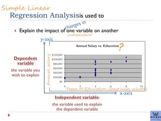
- 1. Regression Analysis Explain the impact of one variable on another Independent variable: the variable used to explain the dependent variable Dependent variable the variable you wish to explain is used to x-axis y-axis Simple Linear independent Annual Salary vs. Education $0 $20,000 $40,000 $60,000 $80,000 $100,000 $120,000 0 2 4 6 8 10 Annual salary Years of Education (past high school) ?
- 2. Regression Analysis Independent variable Dependent variable is also used to x-axis y-axis Simple Linear Quantify linear relationships …develop an equation for the… Y = mX + b value of Y when X = 0 change in Y relative to a change in X Y = b1X + b0 slope intercept The purpose of regression analysis is calculate estimates of the slope and intercept.
- 3. Regression Analysis Independent variable Dependent variable is also used to x-axis y-axis Simple Linear Quantify linear relationships …develop an equation for the… Y = mX + b value of Y when X = 0 change in Y relative to a change in X Y = b1X + b0 slope intercept The purpose of regression analysis is calculate estimates of the slope and intercept. =INTERCEPT(y-range, x-range) =SLOPE(y-range, x-range) using LEAST SQUARES ESTIMATION
- 4. Linear Regression Example Scatterplot House price model: scatter plot 0 50 100 150 200 250 300 350 400 450 0 500 1000 1500 2000 2500 3000 Square Feet House Price ($1000s) (1) Describe the relationship… r = 0.762
- 5. House price model: scatter plot and regression line y = 0.1098x + 98.248 0 50 100 150 200 250 300 350 400 450 0 500 1000 1500 2000 2500 3000 Price in $1000s sqft Selling Price vs. Square Feet trendline (2) Model the Data… Calculate the regression coefficients and interpret b0 is the estimated mean value of Y when the value of X is 0 (if X = 0 is in the range of observed X values) Because the square footage of the house cannot be 0, the Y intercept has no practical application. slope intercept
- 6. House price model: scatter plot and regression line y = 0.1098x + 98.248 0 50 100 150 200 250 300 350 400 450 0 500 1000 1500 2000 2500 3000 Price in $1000s sqft Selling Price vs. Square Feet trendline (2) Model the Data… Calculate the regression coefficients and interpret b1 measures the mean change in the average value of Y as a result of a one-unit change in X The mean value of a house increases by 0.1098($1000) = $109.80, on average, for each additional one square foot of size slope intercept
- 7. y = 0.1098x + 98.248 R² = 0.5808 0 50 100 150 200 250 300 350 400 450 0 500 1000 1500 2000 2500 3000 Price in $1000s sqft Selling Price vs. Square Feet (3) Evaluate the Model… Calculate R2 58% of the variability in the PRICE of a home is exaplined by using the SIZE of the home.
- 8. Standard Error of Estimate The standard deviation of the observations around the regression line. When predicting, this is the stdev of the predictions (3) Evaluate the Model… Calculate R2 and std error
- 9. y = 0.1098x + 98.248 R² = 0.5808 0 50 100 150 200 250 300 350 400 450 0 500 1000 1500 2000 2500 3000 Price in $1000s sqft Selling Price vs. Square Feet (3) Evaluate the Model… Calculate R2 and std error SYX=41.33