This white paper discusses what you need to know when evaluating the performance of solid-state storage systems.

1. Whitepaper
Considerations for Testing
All-Flash Array Performance
What you need to know when evaluating the
performance of Solid State Storage Systems
Abstract
This whitepaper explains important considerations when
evaluating All-Flash Arrays (AFAs). Today, AFAs are typically
deployed to meet stringent performance demands and service
important applications. Flash arrays use new technology with
fewer mature practices to aid evaluation, and flash can behave
in unfamiliar ways. The reader will be in a stronger position to
make the right choice after completing this paper.
August, 2013

2. Copyright © 2013 EMC Corporation.
All Rights Reserved.
EMC believes the information in this publication is accurate as
of its publication date. The information is subject to change
without notice.
The information in this publication is provided “as is.” EMC
Corporation makes no representations or warranties of any kind
with respect to the information in this publication, and
specifically disclaims implied warranties of merchantability or
fitness for a particular purpose.
Use, copying, and distribution of any EMC software described in
this publication requires an applicable software license.
EMC2, EMC, the EMC logo, Symmetrix, VMAX, VNX, Isilon, FAST,
Xtrem, XtremIO, XtremSF, and XtremSW are registered
trademarks or trademarks of EMC Corporation in the United
States and other countries. For the most up-to-date listing of
EMC product names, see EMC Corporation Trademarks on
EMC.com.
VMware and vSphere are registered trademarks or trademarks of
VMware, Inc. in the United States and/or other jurisdictions. All
other trademarks used herein are the property of their respective
owners.
Part Number H12116
2

3. Table of Contents
Executive summary .................................................................................................... 4
Flash is different than disk ......................................................................................................... 4
Audience .................................................................................................................................. 5
Overview of the Paper ................................................................................................................ 5
Background .............................................................................................................. 6
Key Concepts ............................................................................................................................ 7
Testing Tools ........................................................................................................................... 10
Test Plan Primer .......................................................................................................12
Consistent Random Performance .............................................................................................. 12
Functional IOPS ....................................................................................................................... 13
What Knobs to Turn and Outstanding IOPS ................................................................................ 13
Randomness....................................................................................................................... 13
Read/Write Mix ................................................................................................................... 13
Outstanding I/Os ................................................................................................................ 14
I/O Size .............................................................................................................................. 15
Size of LUNs........................................................................................................................ 15
Number of LUNs .................................................................................................................. 16
What to Graph and How to Read the Plots.................................................................................. 16
IOPS (Throughput) and Array Saturation ................................................................................ 16
Consistency ........................................................................................................................ 19
Configuring the Array for Testing .................................................................................22
Preparing the Array for Testing ....................................................................................25
Characterizing Array IOPS and latency..........................................................................27
Basic Characterization ............................................................................................................. 27
Expected Patterns and Observations ......................................................................................... 28
Scaling Performance ................................................................................................................ 29
Sequential Performance ........................................................................................................... 31
Number of LUNs ...................................................................................................................... 33
Read/Write Mix ....................................................................................................................... 34
Characterizing Data Efficiency.....................................................................................35
Evaluating Inline Deduplication ................................................................................................ 35
Post-Processed Deduplication .............................................................................................. 37
Evaluating Actual Raw to Usable Ratios ..................................................................................... 38
Characterizing Consistency ........................................................................................40
Degraded System Performance ................................................................................................. 43
Drive Failures ...................................................................................................................... 43
Controller Disruptions and Failures ....................................................................................... 43
Characterizing VMware VAAI Capabilities .....................................................................45
Preparing the Test Environment ................................................................................................ 45
Evaluate the XCOPY Capabilities ............................................................................................... 45
Evaluate the WRITE SAME Capabilities ...................................................................................... 46
Evaluate Atomic Test and Set Capabilities ................................................................................. 46
Conclusion ..............................................................................................................48
Next Steps ...............................................................................................................48
References ..............................................................................................................49
Appendix A – Prioritized Test Matrix ............................................................................50
Appendix B – XtremIO Configurations ..........................................................................51
3

4. Executive summary
Virtual servers, cloud-based platforms, and virtual desktops are becoming the
standard way to deploy new infrastructures. This trend toward consolidating many
different applications onto a single set of systems causes what is sometimes called
the “I/O Blender” effect. The storage workloads become in the aggregate highly
random and simultaneously distributed across a large percentage of the storage
capacity. At the same time, powerful analytics are driving value for organizations and
placing a premium on the ability to collect and analyze huge volumes of data.
Traditional storage systems using spinning disks and caching controllers are a great
fit for workloads that have manageable working sets and a high percentage of
sequential accesses. In those scenarios, traditional architectures provide the best
value. But for many deployments dedicated to consolidated infrastructure and high
performance analytics, all-flash arrays are a better fit and provide a superior ROI
because they address the highly random access demands of consolidated
infrastructures in a cost effective manner.
Flash storage isn’t new, but recent improvements in price and performance have
made it possible to deploy flash-based storage to meet demanding enterprise
requirements. Flash packaged as standard SAS and SATA drives (solid state drives or
SSDs) has rapidly improved and turned into a generally trustworthy commodity.
Storage vendors have been quick to take advantage, but many are just replacing
spinning disks with SSDs. This doesn’t take advantage of flash’s strengths or
compensate for weaknesses. In the marketplace, some solutions are better at
delivering on the promise of flash than others.
Flash is different than disk
Traditional disk subsystems are optimized to avoid random access. Array controllers
have evolved at the rate of Moore’s Law. Over the last 20 years CPU power and
memory density has improved by a factor of 4,000, while disk I/O operations per
second (IOPS) have only tripled. To make up for this gap, storage engineers use
complex algorithms to trade CPU cycles and memory capacity for fewer accesses to
the underlying disk subsystem of their arrays.
Testing traditional storage focuses on characterizing array controllers and caching.
Those are differentiators for disk arrays, and all tend to be limited by the same set of
commodity disk technologies when it comes to actually accessing the disk.
Flash is an inherently random access medium, and each SSD can deliver more than a
hundred times the IOPS of enterprise class hard disk drives. Enterprise SSDs deliver
consistent low latency regardless of I/O type, access pattern, or block range. This
enables new and improved data services that are only now starting to mature in the
marketplace. However, SSD reads are faster than writes. Flash also wears out, and
endurance will be compromised if the same flash locations are repeatedly written.
This calls for a fundamental rethinking of how controllers for All-Flash Arrays (AFAs)
should be designed, and consequently how those designs should be tested to
highlight strengths and weaknesses.
4

5. This whitepaper explains important considerations when evaluating AFAs. Flash
arrays use new technology with fewer mature practices to aid evaluation, and flash
can behave in unfamiliar ways. The reader will be in a stronger position to make the
right choice after completing this paper.
Audience
This whitepaper is intended for technical decision makers who are evaluating the
performance of All-Flash Arrays, and engineers who are developing test plans and
benchmarking scripts to implement the evaluation tests.
Overview of the Paper
This paper starts with some background on flash storage, All-Flash Arrays, and
testing. Following that, it recommends ways to configure the AFA and prepare it for
testing. The next four sections focus on characterizing AFA IOPS and latency, data
efficiency capabilities, consistency of response, and finally the ability to support
virtual infrastructures at high performance levels. The paper concludes with a
summary and some suggested next steps.
5

6. Background
Flash is a fundamental media technology. By themselves, flash chips can’t do much.
Flash storage solutions in the Enterprise come packaged in many forms:

One of the lowest latency flash solutions places chips on a PCIe card that
plugs directly into the server. EMC® XtremSF™ is a leading example. Server
flash gives applications very fast access to storage. The challenge is having
good software (like the XtremSW™ Suite) to manage card contents.
Additionally, sharing the contents of the flash between servers requires
complex software and fast interconnects.

The next step is to wrap the flash in an external appliance that can be shared
among several servers using standard protocols. These appliances tend to
have minimal enterprise storage features and focus on providing low latency
access to basic LUNs. Flash appliances tend to be built from custom flash
modules that are plugged into the appliance like memory or mezzanine cards
into a server.

All-Flash Arrays provide enterprise storage features such as high availability,
thin provisioning, and deduplication (dedupe). AFAs tend to be built from
SSDs with disk interfaces and hot-plug carriers that make it simple to swap
failed components. The EMC XtremIO™ array uses innovative software and
new algorithms on standard hardware to deliver levels of real-world
performance, administrative ease, and advanced data services for
applications.

Hybrid storage arrays use traditional spinning disks in combination with flash
devices. The flash typically acts as an extension of the controller cache
hierarchy, and much of the innovation revolves around how to manage data
placement between the various tiers. EMC offers SSD storage for Symmetrix®
VMAX®, EMC VNX® Series, and the EMC Isilon® platforms, both as persistent
storage and as media for Fully Automated Storage Tiering (FAST™).

Server SSDs are another popular option. Commodity SSDs are directly
attached to servers, and then managed by the server OS via RAID or tiering
algorithms if available.
EMC provides the most comprehensive portfolio of storage technologies on the
planet, and has a fully developed vision of where flash lives in the data center. As
Figure 1 shows, there is an important role for flash in many parts of the storage
landscape. Tying all those technologies together and orchestrating them in simple,
manageable, and scalable ways is equally critical. Only EMC provides the breadth of
products and vision to make this a reality today.
6

7. Figure 1 Where Flash Lives in the Data Center
This paper focuses on All-Flash Arrays, represented as the second tier from the left in
Figure 1. Any mention of storage and technologies in this paper should be read in the
context of AFAs. Other technologies in EMC’s portfolio are covered in other papers
available at http://www.emc.com.
Key Concepts
Let’s explore a little industry history and set some context before diving into the
actual concepts.
One of the key questions faced by early flash array developers was whether to use
SSDs with standard storage interfaces like SAS or SATA, or custom flash modules that
could appear as storage, memory, or some other device using custom drivers. Some
developers chose to leverage standardized SSDs, while others built around custom
flash modules tailored to a single vendor’s specifications.
Using custom modules allowed for greater integration and potentially improved
performance and density. The down side was that the vendor was now responsible for
all the work and innovation that went into the modules. This was the preferred
approach when the entire flash industry was new and only a few understood how to
best leverage flash media. However, leading enterprise SSD manufacturers have
caught up and in some cases surpassed what is possible with internally developed
flash modules.
Using custom modules is effectively betting against the entire SSD industry:
companies with decades of experience building enterprise logic and media chips
(e.g., LSI, Hitachi, Marvell, Intel, etc.), and SSD startups that attract some of the best
engineers in their fields. Using SSDs adds some latency to I/O path (compared to
PCIe attached flash), but AFA engineers get to select best of breed SSDs and leverage
the rapid innovation and constantly improving reliability in the SSD industry. XtremIO
relies on an industry of skilled suppliers rather than betting on outsmarting them.
7

8. Thus XtremIO focuses on developing the richest software stack, not optimizing flash
device hardware.
With that context, let’s examine a number of flash concepts that are critical to
understand when evaluating AFAs:

Flash is an inherently random access medium. The biggest obstacles to getting
more IOPS from a spinning disk are seek times and rotational delays. To do a
random I/O, the disk needs to first position the read/write head on the correct
cylinder (called a “seek”), and then wait while the disk rotates to the correct
sector. Flash accesses just need to specify the desired address and the correct
location is accessed directly. This means that access time and latency is
consistently low, regardless of where the requested data resides in the SSD’s
logical address space. They’re also consistently low whether the subsequent
requests access sequentially or randomly placed addresses.

SSDs and flash modules are complex all by themselves. Flash media is
passive and needs additional intelligence to become a storage device. All
these devices require a CPU (controller ASIC or FPGA), cache memory, onboard
I/O logic, internal data protection algorithms, and active power management.
These components work in concert to address the concepts covered below.
Some manufacturers do a much better job than their peers in terms of
reliability, performance, and continual improvements. Many functions at the
device level are also present at the array level. Sometimes an array augments
and multiplies the capabilities of the device. Other times, an array assumes
that the devices can’t be trusted and that it needs to compensate for their
possible shortcomings. XtremIO prefers to qualify trustworthy SSDs and
generally lean on their capabilities. Of course the array also makes sure any
hiccups or failures at the SSD level are correctly managed.

Flash writes are more work than reads. Reading the contents of flash is a quick
and simple operation. The address and required length of data is requested,
and the device CPU reads the contents of specified cells and returns them to
the requestor. Writes require the flash cells to be programmed with new
values, take longer to complete, and typically can only operate on larger
sections of the media. If the operation partially over-writes a section, the
contents must first be read, merged in the device’s memory with the new data,
and then written to a new blank section. If no blank sections are standing by,
then the device must first find and erase an unused section. The net impact is
that SSDs typically perform only half to a third as many writes per second as
reads.

Flash wears out eventually. The act of erasing and programming sections of
flash is inherently destructive to the media. The state of cells that haven’t
been written for a long time can eventually degrade, so SSDs sometimes
refresh their contents through additional writes. SSDs compensate for this in
various ways, but eventually all SSDs will wear out with use. Arrays should be
designed to minimize writes to flash, and one of the most effective ways to do
8

9. this is to avoid writing duplicate data (inline deduplication), plus implement
smart data protection that minimizes parity-related writes.

Not all flash is the same. Flash and SSDs are built and priced based on their
performance and endurance. Single-level Cell (SLC) flash stores a single bit
per cell and each cell can typically be written around 100,000 times before
burning out. Multi-Level Cell (MLC, also known as consumer grade flash, or
cMLC) flash stores two bits per cell and each cell can typically be written
around 3,000 times before burning out. MLC flash also tends to be slower than
SLC. Enterprise MLC (eMLC) flash uses clever techniques to improve speed and
endurance. It can typically be written about 30,000 times before wearing out.

Reserving capacity is a ubiquitous practice and can improve performance.
Writing flash is relatively slow and having large areas of pre-erased cells
mitigates some of the delay. Many flash arrays will reserve some amount of
array’s capacity to improve write performance. Indeed, reserved space is also
prevalent in enterprise SSDs, which contain more internal flash than they
present to the outside world. The problem comes when the user expects the
performance quoted with a mostly empty array, but wants to use all the
capacity they purchased. When testing array performance, the most accurate
expectations come from testing with the array almost completely full. Users
typically target an 80% utilization rate and sometimes go above that. Testing
with the array 90% full is strongly recommended.

Flash Translation Layer (FTL). SSDs implement a software abstraction layer to
make flash act like disk. The device CPU hides all the various clever and
complex operations beneath the FTL. This includes maintaining pre-erased
regions of flash cells, abstracting the logical location of data from the physical
cells which hold it at any point in time, minimizing writes to actual flash, etc.
This is done on the flash device, but there are typically analogous operations
at the array level as well.

Garbage Collection is the process of proactively maintaining free pre-erased
space on the flash to optimize writes. It happens in SSDs and may happen at
the array controller levels (some flash arrays try to prevent SSDs from
performing their own internal garbage collection, preferring instead to utilize
controller-level garbage collection algorithms that the manufacturers feel are
superior). Ideally, garbage collection happens in the background during idle
periods. Consolidated infrastructures operate continuously and may never see
idle periods. In this case, garbage collection may impact production
performance. Testing during continuous load forcing garbage collection to be
active is critical for accurately setting predictable performance expectations.

Wear leveling is an important part of flash operation. Because repeated writes
to a flash cell will eventually burn it out, it’s important to write to all the cells
evenly. This is accomplished by separating logical from physical addresses,
only writing to cleanly erased areas of the flash, and post-processing to erase
the physical locations of data that has been logically deleted or overwritten. At
9

10. the SSD level this happens under the FTL. At the array level, the controller
manages the logical/physical abstraction and post-processing to clean up
stale physical locations.

Write Amplification impacts flash endurance. Because flash cells are erased
and written in large sections, more data may be written to the media than
requested by the user. For example, if the user needs to write 4KB but the write
block is 256KB, the flash device may need to write 256KB due to physical
constraints. At the array level, RAID algorithms may amplify writes by adding
and updating parity. Garbage collection also amplifies writes by consolidating
and moving partial stripes of data in order to free up more space for future
writes. SSDs and arrays work to mitigate this by decoupling logical and
physical locations. They also try to combine many smaller requests into the
same larger write block on the SSD.

Read Amplification impacts array IOPS and latency. In order to boost write
performance, some AFAs lock flash modules or SSDs while writing and do not
allow reads to hit the same devices. Read requests end up either being
delayed or serviced by conducting parity rebuilds, which requires reading all
remaining devices in the redundancy group. A single parity rebuild read
request thus results in N-1 flash device reads, where N is the number of
devices in the redundancy group. This dynamic is called Read Amplification
and may show up on some AFA implementations.

Guaranteed Lifetime Throttling. Some AFAs and SSDs provide a guarantee that
the product will last a certain number of years or TB written. Workloads are
varied and unpredictable, so vendors may assure their guarantee by slowing
down writes to the SSDs. Typically the product initially performs at full speed.
After a percentage of the flash cells write endurance has been exhausted,
writes begin to be artificially throttled (slowed down). It usually starts slowly,
but the closer the cells get to complete exhaustion the more writes are
throttled. The end effect is that performance of the array or SSD can degrade
significantly over the deployed lifetime of the product. If the array is
guaranteed for a specific number of years, ask the vendor whether the
performance should be expected to degrade over time due to throttling.
Testing Tools
Selecting the right tool for evaluating AFA performance is important for getting an
accurate characterization of the system. Most performance testing tools are built
around a workload generator. The generator issues I/O to the system under test and
measures how long it takes to receive a successful response. Several free tools are
available:

IOmeter – The most commonly used option. It’s attractive because it has a
GUI, which makes it simple to get started. But it’s also easy to use IOmeter to
generate inaccurate results, and building complex testing scripts can be more
challenging.
10

11. 
FIO – Very flexible benchmarking framework that runs on Linux. It has the
ability to generate unique data to test in the presence of deduplication and
compression, but doesn’t allow a specific deduplication ratio to be selected.
It’s very easy to script, and lightweight to allow each client to generate many
I/O requests before running out of CPU cycles.

BTEST – High performance and low overhead load generator for Linux. It
doesn’t include all the options and built-in automation capabilities of some of
the other tools. It can generate a very high multi-threaded load with a specific
deduplication ratio. BTEST is a command line tool that’s great for running
quick manual tests, or as the foundation for custom automation.

VDbench – Powerful and flexible load generator that’s been in use for many
years. Available for download through the Oracle Technology Network. It
includes the ability to select deduplication and compression ratios for the
generated I/O. The one downside is that VDbench uses Java and consumes
more CPU on the load-generating client. More client machines may be needed.
Whichever tool is selected, make sure that the array (the “System Under Test”)
becomes the bottleneck during testing. Otherwise, all the extensive testing will do is
highlight limitations in the testing environment. This means that there needs to be
enough aggregate client power to generate a high rate of requests to the array and
measure their responses. Because of various queuing points and limitations, it’s
generally necessary to use multiple clients to gain sufficient parallelism. This is true
even if a single powerful client is available. Aim for at least three test clients,
although the examples in this paper are based on four clients. Similarly, make sure
that the front-end network connecting the clients to the array has enough bandwidth
(port, backplane, and ISL) to carry the necessary load. Creating a test environment
where the array is the bottleneck component will ensure meaningful results.
11

12. Test Plan Primer
Before getting down to the details of testing, consider the context. What are the goals
of the plan below, how do they relate to the nature of flash and AFAs, and why are
they important? This primer helps guide thinking about testing flash arrays.
Consistent Random Performance
Solid-state appliances were once upon a time introduced as very specialized storage
for the most demanding and valuable applications. These appliances were typically
directly connected to a small set of hosts and dedicated to a single application.
That’s changing as the flash market evolves. These days solid-state storage is
everywhere and being widely adopted by organizations of every size as a way of
boosting the value of their consolidated infrastructures. That’s the core of what’s
being explored in this paper.
Interest in Enterprise workloads on consolidated infrastructures focuses this paper on
100% Random I/O. Whether the consolidated infrastructure is managed as a private
cloud or more traditional IT data center, many different applications, departments,
and functions are all using the same underlying hardware and software to meet their
needs. Most applications already have significant random I/O components. When all
these applications are running on the same hardware at the same time, their requests
are blended into a single stream directed at the storage infrastructure. Aggregated
requests become much more random and address a much larger range of capacity.
Even sequential operations like database scans and data warehouse loads end up
being random since many independent users are running these requests at the same
time.
But it goes beyond that. Consolidated infrastructures also demand consistent,
predicable performance and non-stop operation. The performance must be consistent
over the long term and can’t degrade as the storage ages, fills up, or holds different
applications. It must be workload independent. This is so that the service can be
offered with little worry about a particular application’s workload, or whether adding a
strange new application will upset all the existing customers. These infrastructures
need to operate 24/7/365 with little oversight and a skeleton administrative staff.
Nobody is waiting around to react to unruly applications and manually isolate them to
specific controllers or RAID groups. The storage just needs to work as expected no
matter what is running on top. And it needs to do so over the planned operational life
of the storage.
For this reason, the focus is on random performance and 100% random IOPS (in fact,
this is exactly what flash arrays are supposed to excel at). The goals of our test plan
are to probe the array in the context of consistent, predictable, long-term performance
under stressful conditions. This will highlight strengths and shortcomings that are
likely to manifest when deployed in production as part of a consolidated
infrastructure.
12

13. Functional IOPS
The most important factor when evaluating an array is functional IOPS at low
latencies. Functional IOPS represent the real workload performance that customers
can expect in typical operating conditions. Functional IOPS are based on
measurements in the context of how an array will be used in production, not how it
can be shown off in a lab (also known as “hero” numbers). They must be measured
end-to-end at the host. They must be 100% random and accessing previously
overwritten SSDs to reflect steady-state performance. They must be based on nearly
full arrays and access the full address range of large LUNs. They must be a mix of read
and write requests generated at high loads to reflect peak operational periods. This
approach is the foundation for measurements that accurately set expectations of
array performance in production.
In addition, modern storage arrays support a wide range of features and data
services. Users are attracted to those capabilities and consider them when choosing
storage. Those features can impact the performance of the array. When
benchmarking, it’s important to enable all the features and data services intended to
be used in production.
Often functional IOPS and active data services aren’t reflected in vendor-published
performance numbers. One set of features is advertised, but system performance is
reported with many of these valuable features disabled to get a higher number (or
with an unspecified array configuration that might be substantially larger or more
expensive than the configuration being considered). Or the system is configured and
tested in a way that is completely different from how it will be used in production.
When reading vendors’ published performance reports, ask for more details if it’s
unclear what features were enabled or how the array was configured and tested. Final
deployment decisions should only be based on functional IOPS.
What Knobs to Turn and Outstanding IOPS
There are many options for generating load on the array and measuring performance.
Benchmarking tools have many more options and permutations than are practical to
use during any single evaluation project.
Randomness
As discussed above, the recommendation is to focus on 100% random access during
the evaluation. Computing is rapidly transforming toward consolidated infrastructure,
which looks very random to the storage subsystem.
Read/Write Mix
What percentage of requests is read versus write? The recommendation is to test
several mixes where there is a significant percentage of each request type. For
example: 35% Read/65% Write, 50/50, and 80/20. This provides insight into how
array performance will shift with different application mixes.
13

14. Why not 100% read or 100% write? These workloads are mostly of academic interest
and rarely part of real-world environments for AFAs. They are unrealistic because
nobody has that workload on a shared array being used for multiple applications –
the environment that enterprise flash arrays are designed to serve. The other reason
is that pure read workloads hide important AFA processes like garbage collection and
flash locking, so results will look far better than real world. If there is lots of time for
testing and a mature test automation framework, it might be interesting to collect this
data. But in general these workloads are not useful in setting expectations for realworld AFA performance.
Outstanding I/Os
How many I/O requests are issued simultaneously and actively being serviced? The
number of outstanding I/O’s (OIO) is critical. It effectively becomes the main knob for
controlling load level during testing. OIO is determined by two factors: how many load
generator threads are running, and the allowable queue depth per thread. All the
referenced benchmark tools provide ways to control these options.
Figure 2 illustrates the concept of Outstanding I/O’s in the context of the system
under test. There are multiple other queuing points in the system, but the load
generator and testing aims to find the ideal number of generated outstanding I/Os
that result in the best IOPS results below a given latency threshold. Each load
generating client has a number of worker threads, that each have a given queue
depth. The total sum across all clients, threads, and queues controls the number of
outstanding I/O’s in flight against the system under test.
14

15. Figure 2 Outstanding I/O’s at the Load Generator
After the data has been gathered, the OIO-controlled load becomes the basis for two
important graphs: the latency versus IOPS curve and the latency versus outstanding
I/O’s curve. These graphs are presented in the next subsection.
I/O Size
How many bytes are requested in each I/O? The recommendation is to test a small set
of sizes ranging from 4KB to 1MB. Anything smaller is unlikely to be found in
production. Anything larger is likely to represent only occasional phases or edge
cases for applications deployed on flash arrays. If the target applications have
frequent phases where large I/O sizes are present (database loads, backup to tape,
etc.), it may make sense to throw in some orthogonal test phases that focus on these
larger sizes. But for the bulk to the test matrix it generally makes sense to keep I/O
size small when testing flash arrays.
Size of LUNs
How large is each LUN being accessed? Addressable capacity in spinning disk arrays
is very large and only a small fraction tends to be active. AFAs have much smaller
capacities that tend to be mostly active. The recommendation is that the total LUN
capacity tested be much larger than the cache in the array controllers (at least 10x).
Ideally close to the full capacity of the array. Otherwise, a big percentage of the
requests are likely to address cache memory and not represent the steady state
15

16. performance in production, consolidated infrastructures. As detailed later, the
recommendation is to size the LUNs so that each LUN represents 5% of maximum
addressable capacity. This allows us to precondition the array and then start testing
realistic performance with minimal effort.
Number of LUNs
How many LUNs (volumes) are being accessed at the same time? The
recommendation is testing multiple LUNs, and paying attention that the load on each
LUN is roughly equal across all paths to the LUN. With each LUN covering 5% of the
array capacity, the array will end up holding 20 LUNs. The plan is to delete two of
those LUNs and create 10% empty space as additional working room for the array.
The remaining 18 LUNs will be accessed in different numbers as part of the test
matrix. This is to assess how the performance changes when the array needs to
manage different numbers of LUNs and address different percentages of capacity.
If the target application will use many smaller LUNs, then consider starting with that
configuration. For example, create 200 LUNs, each representing 0.5% of addressable
capacity. Do this as part of preconditioning the array so that the LUNs already exist
and testing can commence as soon as the array is conditioned.
What to Graph and How to Read the Plots
IOPS (Throughput) and Array Saturation
After the data has been gathered, the OIO-controlled load becomes the basis for three
important graphs:
1. Average Latency versus IOPS – Illustrates how average latency increases as
the array delivers more IOPS for a given workload. The flatness of the curve is
an important indicator of performance and consistency. The point at which the
latency curve crosses various thresholds indicates the IOPS that can be
expected at that latency level. Where the curve begins to rapidly curve
upwards is called the elbow (or knee) of the curve and is the region where the
array is reaching its limits. It can be though of as the redline for that particular
array and workload. Plotting multiple curves for different workloads or arrays
lets evaluators quickly draw a visual comparison between their relative
16

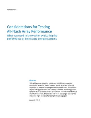
17. performances. Figure 3 is an example of this curve with highlighted features.
14
Response Time versus IOPS
Storage 1
8
10
Storage 3
4
6
El bow of t he Curve
0
2
Response Time (milliseconds)
12
Storage 2
0
5000
10000
15000
20000
25000
IOPS
Figure 3 Latency versus IOPS
2. IOPS versus OIO – This curve shows how the system responds to requests for
additional load. This is roughly analogous to the horsepower versus RPM
graphs in automotive magazines. The ideal graph will have a long region with
bar heights up and to the right. The region where subsequent bars start to
flatten out is the knee of the curve and represents the outstanding I/O level at
which the system is reaching its limits. If the bars start back down at some
point, it means the array has become overloaded. This is an important
indicator: the infrastructure should be sized so that arrays are rarely operating
in an overloaded state. Figure 4 shows an example of this graph using bar
heights to represent the IOPS at discrete OIO values.
17

18. 212174
211462
256
320
200979
150512
89712
46757
23887
0
I/O's per Second
50000 100000
200000
IOPS versus Outstanding I/O's
8
16
32
64
128
Outstanding I/O's
Figure 4 IOPS versus Outstanding I/O's
3. Average Latency versus OIO – Illustrates how average latency increases as the
load on the array increases. This has a direct correlation to Figure 3, but is in
terms of a factor controlled in the benchmarking. The graph provides insight
into the number of outstanding I/O’s that the array can tolerate before being
saturated. Look for the same features as in the Latency versus IOPS curve, and
the expect it to have an inverse shape compared to Figure 4. Figure 5 shows an
example of this graph using bar heights to represent the average latency at
discrete OIO values. Notice how at 128 outstanding I/O’s the latency begins to
climb rapidly (Figure 5) while the IOPS begins to flatten out (Figure 4). The
combination is a strong sign that the array is reaching its saturation point in
18

19. terms of outstanding I/O’s.
Figure 5 Latency versus Outstanding I/O's
It may be helpful to group multiple workloads, multiple arrays, configurations, etc. on
the same graph to visually compare performance. These graphs are the simplest and
most powerful decision tools to use during the evaluation process.
Consistency
In addition to the three primary graphs, additional graphs based on detailed interval
measurements are very useful for understanding the consistency of array
performance. This is important for delivering high quality user experiences.
To generate these graphs, the average latency statistics need to be collected every
few seconds during representative workload runs where the array is fully saturated.
The next section provides more details on how to do that. For now, assume the target
workload and load level has been identified based on the graphs above. Run that test
for an extended period (at least an hour), collecting latency statistics for each LUN or
thread every 5 seconds. Throw away the first few minutes of the results gather while
the benchmark was warming up. Once that data has been collected, generate the
following two graphs:
1. Latency versus Time – Draw time (or measurement number) on the X-axis and
plot a point for the interval’s latency measurement on the Y-axis. The ideal
graphs will show smooth lines for average latency. Use these graphs to get a
feel for the relative performance consistency of the various arrays being
19

20. evaluated. Figure 6 shows an example of what one of these graphs might look
like. In this particular example, the array undergoes some preconditioning and
begins to show higher average latency over time.
Figure 6 5-Second Average Latency versus Time
2. Latency Histogram – Plot histograms of the average latency measurements.
This is another way to summarize the behavior of the array in a single familiar
graphic. To compare multiple arrays, overlay their histograms using different
colors or just display them side-by-side. Figure 7 shows an example of what
one of these graphs might look like.
20

21. 0
1000
Frequency
2000
3000
Latency Histogram
0.0
0.5
1.0
1.5
I/O Latency (milliseconds)
2.0
2.5
Figure 7 Latency Histogram
Using these graphing techniques the evaluator can quickly develop deep insights into
the expected performance of the arrays being tested and be in a strong position to
decide which is the best fit for the organization.
21

22. Configuring the Array for Testing
The first step in the evaluation process is to install and configure the arrays under
test. The actual process will be different for each array. The general guidance is to
follow the vendor’s best practices as long as they keep the results reasonably
comparable. If the best practice forces the arrays to be configured differently, note
the differences and consider them during the evaluation process. For example, if one
array is configured with a 60% raw-to-usable capacity ratio and another is 80%, be
sure to consider these factors during the evaluation and final decision process.
That said, all evaluation tests should be run with the full range of array services
enabled:

Make sure the data protection level is set to N+2 redundancy (or equivalent) to
ensure data is protected from SSD or flash module failures.

If the array supports high availability across multiple controllers, ensure it’s
configured according to best practices.

Enable any data efficiency services like thin provisioning, deduplication, and
compression.

Configure the fastest connectivity practical for the environment. For example, if
there’s a choice between Fiber Channel (FC) and iSCSI, use FC for the tests.
Configure multiple paths between the clients and array. Make sure the
switches used during the testing will be able to support the additional load
and not become a bottleneck.

Configure the client-side HBA tuning parameters and multipathing according
to the array vendors’ best practices. Often AFAs perform better with flashspecific tunings, since the HBA defaults are typically set based on traditional
spinning disk arrays.

Configure client-side parameters related to timing. Most clients have BIOS
settings that control two relevant parameters. Setting both these options will
help gather accurate measurements during the evaluation:
1. Power Management – The first is power management, which allows the
server to slow down its CPUs (and sometimes other chipsets) to save
power. In general this is a great feature, but when benchmarking the
fluctuating chip speeds can result in misleading measurements. Turn off
power management for the duration of the testing and configure the client
machines to always run at full speed. In the BIOS, look for the following
options and set them as suggested below:
a. “Main BIOS Settings”  “Processor C State” – Set to “disabled”
(The system remains in high performance state even when idle)
b. “Main BIOS Settings”  “Processor C1E” – Set to “disabled”
(The CPU continues to run at its maximum frequency in C1 state)
22

23. c.
“Main BIOS Settings”  “Package C State Limit” – Set to “c1”
(When the CPU is idle, the system slightly reduces the power
consumption. This option requires less power than C0 and
allows the server to return quickly to high performance mode)
2. Timer Precision – By default, many clients (especially older machines) are
configured with event timers that tick at the 10-millisecond frequency. This
isn’t sufficient resolution when trying to measure flash array events that
typically happen in less than a millisecond. Newer machines include a
High Precision Event Timer (HPET) that sometimes needs to be enabled in
the BIOS and the operating system. Ensure that the HPET is active and
available to the benchmarking application.

Pay attention to LUN access models. How LUNs are accessed is related to the
High Availability (HA) and scaling models used in the array architecture. Refer
to Figure 8 to see the variety of options in use today. AFAs are similar to disk
arrays in that they offer active/passive, dual-active, active/active, and N-way
active HA models. In addition, the array may employ a scale-up, aggregated,
or full scale-out model for system expansion. The access paths and
performance available to any particular LUN will vary based on these models.
The same is true for port mapping best practices. Configure initiators to
access LUNs through as many controllers and paths as possible for each
array’s access model.
Figure 8 High Availability Access Models
23

24. In general, if a feature shows up on the glossy brochure make sure that it’s enabled
during the test. If a vendor recommends best practices for tuning clients and
switches, incorporate those best practices into the testing. That will give a true
reflection of performance in production. If the best practices wildly diverge between
vendors, it may be necessary to test one vendor at a time and change the parameters
on the client between test phases.
It’s important to test with all data services enabled. If the array has been designed
around flash and advanced data services, enabling those services should result in
almost no degradation or possibly even improve the reported performance. But arrays
that retrofit flash into an older design will show measurably lower performance.
Arrays that simply replaced spinning disks with SSDs are very likely to amplify writes
and exhibit performance anomalies with write-heavy or mixed workloads. This will
result in overall lower performance (and flash endurance) as the array does more
back-end I/O to the disks. Retrofit architectures also depend on a large percentage of
the I/O fitting in the array controller cache. Fully random workloads are more
prevalent in today’s real-time, shared, and virtualized data center. Retrofit
architectures tend to display high latencies and controller bottlenecks when
challenged with fully random workloads. These weaknesses can be revealed when
testing for functional IOPS.
24

25. Preparing the Array for Testing
The next phase is to prepare the array for testing. This is uniquely important for AllFlash Arrays. Fresh out of the box, flash behaves in a way that doesn’t reflect steady
state, long-term operation. Flash arrays tend to perform better when new/empty and
some vendors will publish benchmark numbers in this state. This performance cannot
be maintained once the array has been written over completely and no longer
contains empty/zeroed-out flash pages. This is called the “write cliff”. Similarly, flash
arrays and SSDs always need to place new data in a free location (sometimes called
“allocate on write”). When the array is mostly empty, free space is easy to find and
measured performance may look higher than what’s likely during production. The
process of recycling locations that are no longer referenced so they may be used for
new writes is the aforementioned garbage collection, which may have adverse affects
on array performance, and can be witnessed during testing by preconditioning the
array and then writing new information as the array fills up.
To get meaningful results, the array first needs to be prepared by overwriting all the
flash cells several times. This is often called “preconditioning” and simulates how the
array will perform after it has been in service for a long time. Capacity utilization is
also important, since having lots of free space means the array doesn’t have to work
hard to find new places for incoming data. In production environments, operating
with the array at least 80% full leads to the best asset utilization. The
recommendation is to test the array at 90% full levels: there will invariably be times
when the array holds more data than the target utilization level. This is especially true
for environments without TRIM, as arrays will eventually fill up all logically
provisioned space. With thin provisioning, that means 100% of the allocated
physical space will be filled. Lastly, AFAs need to be prepared with tools that generate
unique uncompressible data. All the tools mentioned earlier have options that will
work.
The simplest way to prepare the array is to create multiple LUNs during the
preconditioning, and then delete some LUNs to free up 10% of the space for testing.
For example:
1. Create 20 LUNs, each taking up 5% of the available capacity. For example, let’s
say that there’s 8,000GB available after configuring the array according to best
practices. In this case, create 20 LUNs of 400GB each.
2. Map those LUNs to the hosts (test clients) used for the testing. For
preconditioning, the most efficient option is to divide the LUNs among available
hosts. That way, each host is responsible for preconditioning a portion of
addressable storage. Attach the LUNs to the host OS and do a little I/O to each
LUN from the host to make sure they are accessible.
3. Pre-condition the array by overwriting each of the LUNs three times using unique,
uncompressible data. In our example, if each LUN is 400GB, ensure that at least
1,200GB of unique uncompressible data are written to each LUN. Do this by
setting the test tool to issue large block (e.g., 64KB) sequential writes to each
LUN. Use one thread/process per LUN to keep the I/O stream sequential. Set the
25

26. thread queue depth to something large like 32. Some of the tools have
parameters that allow the amount written to be set explicitly (e.g., maxdata=nnn
for VDbench). This option makes stopping the preconditioning process simple. If
the tool doesn’t have this capability, monitor the steady-state I/O rate and
estimate how long the process needs to run to guarantee each LUN is overwritten
at least three times.
Why overwrite the LUNs three times? Why not just write all the capacity once and
be done with it? The reason to write more is that flash arrays have internal
reserved capacity (sometimes called the “performance reserve”). SSDs also have
internal reserved capacity. Both these reserved capacities (sometimes as much
as an additional 40% of capacity) needs to be included in the preconditioning.
This ensures that all flash cells in the system have been written at least once and
the garbage collection mechanisms are actively working at both the SSD/module
level and the system level. This is the expected condition during long-term
production deployments.
Preconditioning is also a good place to verify the real usable capacity of the array.
If the array states that it has 10TB free, use that value to set the maximum data
parameter or run time. If the array runs out of space before the preconditioning
completes, the reported capacity isn’t accurate. Some arrays pre-allocate
overhead for metadata and RAID, while others allocate it on demand and initially
report overly optimistic capacities.
4. Once pre-conditioned, delete two of the LUNs marking 10% of the array as free. In
our earlier example, the array has 8,000GB full of data. By deleting two of the
400GB LUNs, the array will be left with 7,200GB of data in 18 LUNs and 800GB of
free space (10%). Do this by unmapping the LUNs from the hosts and deleting
them via the array UI.
As soon as pre-conditioning completes and 10% of the space has been freed up,
immediately start testing as described in the next section. It’s important to avoid
idling the array and giving garbage collection time to scrub the free space.
Deployed in consolidated infrastructures, arrays will rarely be idle and garbage
collection needs to be able to work during user I/O.
Contrast the above approach with benchmark tricks deployed in the industry. Some
vendors publish benchmark results using a mostly empty array. They address only a
small slice of available capacity to maximize the controller’s caching benefits. One
clue to this game is explanations along the lines of “application working sets are
relatively small, so we don’t need to test with large LUNs and full arrays”.
26

27. Characterizing Array IOPS and latency
The focus of this section is on core characterization of the array. This section is
organized around a number of phases that are useful for evaluating array
performance.
Basic Characterization
Combining recommendations from previous sections, the test matrix might be
summarized as all the permutations of parameters in Table 1 below:
Test Parameter
Access Pattern
Size of LUNs
Read/Write Mix
I/O Size
Number of LUNs (LUN#)
Outstanding I/O’s Threads
Outstanding I/O’s Queue Depth
Value
100% Random
5% of physical capacity per LUN, with 18 full LUNs
populated using unique uncompressible data. The
system should have less than 10% free space.
35% Read/65% Write, 50/50, 80/20
4KB, 8KB, 64KB, 1MB
6, 12, 18
LUN#, 4xLUN#, 8xLUN#
1, 4, 16, 32
Table 1 Test Matrix Summary
If exact features of the environment are known, substitute those values for the ones
in Table 1. For example, if the application read/write mix is actually 73% Read/27%
Write, then use that value instead of the suggested 80%/20% values. The test matrix
is a suggested starting point that can be customized to meet specific needs. If the
values are customized, make sure to keep the coverage equally complete. Don’t
compromise on important stress points like keeping free space at 10% or less.
For all these tests:

Set the load generator to write unique, uncompressible data to ensure full
writes to the underlying storage. For well-designed deduplication systems, this
will represent worst-case performance since this drives the maximum amount
of data I/O to the SSDs.

Run each test instance long enough to reach steady state IOPS. Based on our
experience this should be at least 300 seconds, but 600 seconds are
recommended. This is important since it may take multiple threads some time
to all get going, and a new workload may take some time to push the old
workload through the cache and pattern matching algorithms.

Script the tests to go from one test to the next. This prevents the array from
idling for too long and giving garbage collection algorithms time to reclaim free
space. As mentioned previously, keeping the garbage collection system under
pressure is important for getting a clear picture of how the array will perform
long-term under constant load.
27

28. 
Pay attention to the latency of the results, and how it changes as the load
increases with added threads and queue depth. Latency is expected to
increase exponentially as the array reaches its limits, but flash array latency is
most meaningful in the region below 1 millisecond for typical small random
accesses. Above that, latency will rapidly explode to unusable values for
typical flash array applications.
At 300 seconds per test, the above example matrix should take approximately 27
hours to complete. As the tests finish save the results in a file. Then import them into
a spreadsheet or database for analysis. It’s easiest to see patterns and behavior
when summarized and graphed as described in the Primer section on page 12. Tools
like Microsoft Excel or the R Project for Statistical Computing are very useful for
analyzing benchmark results.
Expected Patterns and Observations
Most AFA performance trends should resemble patterns for more traditional spinning
disk arrays. Here’s a summary of what testing is likely to uncover after graphing the
collected data:

As the number of outstanding I/O’s increase, IOPS will increase rapidly while
latency remains relatively low. Once the array becomes saturated, IOPS will
increase slowly or decrease while latency increases rapidly. Pay attention to
the maximum latency. For an AFA, most of the latency curve should stay below
1 millisecond. The maximum usable latency for random access applications
on flash arrays is likely below 3-5 milliseconds. Any IOPS achieved at higher
latencies isn’t meaningful. Look for the elbow of the curve where latency starts
to increase rapidly. The corresponding number of outstanding I/O’s is likely
the saturation point for that workload.

Increasing I/O sizes will generally lead to higher MB/s throughput and higher
per-I/O latency. At large I/O sizes (e.g. 64KB), the array may become
bottlenecked on some internal component like the disk controller or PCIe bus.
This is more likely for older architectures that retrofit spinning disk arrays with
SSDs. The SSDs themselves are unlikely to be the bottleneck unless there are
very few SSDs per array controller. This may happen with hybrid arrays.
Another sign of legacy architecture is if the array does relatively well at large
I/O sizes, but relatively poorly with smaller I/O sizes.

As the percentage of write operations in the mix increases, aggregate IOPS will
decrease. Write operations tend to be inherently slower than reads for SSDs,
and will periodically invoke garbage collection processes, which amplify writes
(as the process re-packs data in order to free up space for incoming writes).
The observed decrease should be proportional to the capabilities of the
underlying SSDs. Remember that the IOPS difference at varying write
28

29. percentages isn’t linear. Not only are reads generally accessing fewer flash
cells, but write activity can lock out readers and reduce read IOPS.

If garbage collection has a significant performance impact, the results of any
test where garbage collection activates may be confusing. For example,
plotting latency as a function of IOPS may show regions where latency and
IOPS fluctuate rapidly like in Figure 9. Such curves are a sign of caution: The
array may demonstrate unpredictably poor performance under continuous
load – precisely when consistent performance is most important.
Figure 9 Garbage Collection Impacts Performance

Table 3 in Appendix A on page 50 illustrates how to organize the resulting
data. The table also highlights regions organized in terms of priority for the
testing. If there isn’t sufficient time for testing, the tester can follow the priority
guidelines in Table 3. Use the priorities to gather the most meaningful data
first, and gather lower priority data points as time permits.
When characterizing XtremIO arrays, consult Table 4 in Appendix B on page 51 for
LUN sizes and other configuration recommendations. The table is arranged based on
the number of X-Bricks being tested.
Scaling Performance
An important orthogonal factor to consider is scaling. Most long-lived applications
and infrastructures will eventually need more storage. “More” can mean greater
capacity, higher IOPS, or lower latency at high loads.
There are typically three ways that systems are scaled:
29

30. 1. Forklift – A larger, faster system is installed, the data is somehow migrated
from the old system to the new, and the old system is eventually removed or
repurposed for a less demanding use. In the Flash segment, appliances with
fixed performance and no ability to scale tend to fall into this category.
2. Scale-Up – Adding additional shelves of disks to existing controllers to grow
the existing system. Or replacing existing controllers with more powerful
controllers. The capability of any single system is typically limited to a single
HA pair of controllers and the maximum number of disks supported behind
those controllers. If applications need even more capacity or performance,
then administrators need to install and manage multiple systems and
distribute application data among them. Many scale-up architectures are
also dual-active (Figure 8) across HA controllers, meaning that each volume
is serviced by a single primary controller during normal operations.
3. Scale-out – The storage system is architected as a multi-node cluster of many
controllers working in concert to service application demands. Growing the
system involves adding more nodes (and usually disks) to the existing
cluster. In true scale-out designs, the new resources become available to
service new as well as existing data, and the full power of the system grows
in proportion to the nodes in the cluster. Some vendors label aggregated
architectures as scale-out. These are more of a hybrid scale-up design:
components are managed as a single system, but services for a specific
volume are pinned behind a single controller. Growing the cluster allows for
greater aggregated capabilities, but the capabilities for any one LUN or
volume do not change.
It’s important to evaluate scaling strategies, how the storage can be scaled, and what
that scaling means to applications. Consider what can be done if the resources of a
single array or set of controllers becomes a limit. Or a single critical volume needs
more performance. With All-Flash Arrays, scale-out is highly desired since no single
controller is fast enough to unleash the performance of a large group of SSDs.
The ideal solution will be simple to scale with minimal interruption to applications. It
will deliver near-linear increments in performance: twice as many components should
result in roughly twice as many IOPS. Management should be at the system level and
stay constant regardless of deployment size. The full capabilities of the system
should be available to a small number of volumes or able to be distributed with little
overhead among many volumes. Figure 10 uses an EMC XtremIO example to illustrate
ideal scaling for the system, where performance and capacity scale linearly, while
latency remains consistently low. If scaling is a problem, then while capacity
increases linearly, the IOPS will start to flatten out and the latency increase with
added cluster components.
30

31. Figure 10 Linear Scalability with Consistent Low Latency (EMC XtremIO)
During the evaluation process, consider the scaling options are available to support
the organization’s mission. Look at how load is distributed across system
components in different scenarios as the system scales. Is work distributed across
every component, or do some components bear the brunt of the work while others are
mostly idle? Are both front-end requests to the clients and back-end requests to the
SSDs balanced? Are front-end requests grouped to the same small set of back-end
hardware, or can the requests be serviced by the entire system?
Understanding the balance of data requests will provide insight into potential
bottlenecks in the architecture.
Sequential Performance
Even though AFAs are focused on random workloads, understanding sequential
capabilities is useful for a complete picture. Certain phases in the application
workflow (e.g., data load or scans) can apply sequential loads on the system. Of
course remember that if the array is used for multiple applications, sequential I/O
from one application will be intermixed with other application streams, resulting in a
more random overall profile as seen by the array controllers. The goal for this phase
is to discover what combinations of load generator parameters give optimal
throughput. Do this as follows:
1. Start with relatively small I/O size (e.g. 32KB), thread count, and thread
queue depth.
31

32. 2. Run a few short tests (e.g., 300-600 seconds) to measure throughput and
latency, and then increase each of the parameters one at a time and test
again.
3. Graph latency versus outstanding I/O’s (like Figure 5) and latency versus
throughput (like Figure 3 except using MB/s instead of IOPS) for each I/O
size. Based on the graphs, select a set of I/O size, threads, and queue depth
parameters that give high throughput while keeping latency relatively low.
4. Do this for both reads and writes.
These measured values can give insight on how the application can be tuned to
provide the best performance from the array. If the application can’t be tuned, these
tests will show what can be expected from the array during sequential I/O.
20
15
10
5
Latency (ms)
1500
1000
Throughput (MB/s)
2000
25
Sequential Throughput and Latency
Ideal Throughput
0
Ideal Latency
500
Problematic Throughput
Problematic Latency
5
10
20
50
100
200
500
I/O Size (bytes)
Figure 11 Sequential Throughput versus Request Size
Figure 11 shows what might be observed during the sequential testing. The lines in
blue show ideal behavior where the throughput goes up and holds steady, while
latency increases relatively slowly. The lines in green show potentially problematic
behavior, with throughput dropping and latency climbing more rapidly.
Note that latency is generally less critical for sequential performance. What matters
most is the aggregate throughput of data, not how many milliseconds any individual
I/O in that stream takes to complete (video streaming excepted). By its nature,
processing larger I/O requests take longer. The request holds more data to process
and takes longer to transmit and receive each step of the way. Additionally, all arrays
exhibit greater sequential performance when keeping the various queuing points full
of requests. This means the average request ends up sitting longer in queues, and
accumulates more latency before being serviced. Decide on a reasonable latency
32

33. ceiling for sequential I/O applications and use that as the cutoff when measuring
sequential throughput.
Number of LUNs
Another area to explore is how the array behaves with the available capacity divided
among different numbers of LUNs. Ideally, the aggregate performance of the array will
be the same regardless of how the capacity is divided into LUNs. In reality, this is not
always the case. Some arrays associate a large amount of metadata for each LUN,
and deployments of many LUNs limit space for metadata caching and slow down
metadata operations. Arrays can also exhibit internal limitations based on per-LUN
buffers in the I/O path. More simply, some arrays use RAID implementations that limit
LUNs to a particular set of SSDs or flash modules. This makes it physically impossible
to tap into the full power of the hardware without creating multiple LUNs on the array
and using additional tools to “glue” them together.
Some applications will need a small number of large LUNs. Other may prefer a large
number of small LUNs. If time is limited and the array is destined for a specific
application, then structure testing based on the LUN size best practices for that
application. Otherwise, it may be useful to gather empirical measurements of how the
array performs with different numbers of LUNs.
This test plan already includes some LUN number testing and covers testing with 6,
12, and 18 LUNs. This corresponds to 30%, 60%, and 90% of available capacity for
the array. The supplementary testing should focus on the extremes:
1. 4 LUNs – Assign 90% of available capacity to four LUNs, and map those LUNs
to all the test clients. Perform the most relevant set of test measurements,
accessing the four LUNs from all the clients.
2. 128 LUNs – Divide 90% of available capacity into 128 LUNs. Ideally, map all
LUNs to all clients as done for previous tests. If the client OS or initiator
software is limited in terms of how many LUNs can be simultaneously
accessed, divide the LUNs among available clients. For example, if there are
four clients then map 32 LUNs to each client. This makes the access patterns
a little less random, but is likely to reflect how the application will be
accessing the LUNs given the client limitations.
Precondition the array again in the new configuration. This ensures that all the data
and metadata reaches steady state before starting the measurements. Once
preconditioned, immediately start testing. To save time, focus on the workload
setting that resulted in the best performance for the tests done earlier.
Figure 12 shows an ideal and problematic result when testing different numbers of
LUNs. Ideally, a small number of LUNs is able to serve the same number of requests
as the aggregated performance of many LUNs. Some architectures struggle to do this
efficiently, which complicates management and data layout: It forces the application
to distribute data across many smaller LUNs or use additional volume management
software to present the application with a smaller number of aggregated LUNs.
33

34. 250000
250000
100000
IOPS
150000
110000
0
0
50000
50000
100000
IOPS
240000
200000
230000
150000
300000
Problematic Aggregate IOPS vs. # Test LUNs
200000
250000
Ideal Aggregate IOPS vs. # Test LUNs
4
128
# Test LUNs
4
128
# Test LUNs
Figure 12 IOPS versus Aggregate Number of Test LUNs
Read/Write Mix
If the Read/Write mix is critical for the application and actual mix ratios are known,
then substitute that mix for one of the suggested ratios in Table 1 on page 27 during
characterization testing. Additionally, it may be useful to add tests with 100% read
and 100% write access patterns for additional points of comparison.
Be aware that some arrays optimize reads at the cost of writes, and others have
architectures that lock out readers while a writer is active to the same SSD or flash
module. These features will manifest in a drastic drop in IOPS when introducing even
a small percentage (e.g., 10%) of writes into the mix. See the IDC Technology
Assessment for more information on non-linear flash behavior in mixed
environments.
Figure 13 shows one possible scenario: the green line illustrates how the IOPS can
drop off very quickly and non-linearly when even a small percentage of writes are
introduced into the I/O mix. The ideal result (blue line) looks more linear and
predictable based on the 100% read and write measurement and the percent of write
requests in the mix. Even though pure 100% read or write performance may be
higher, there is a wide range of mixed ratios where performance will be significantly
below the ideal. Few applications are purely reads or writes, so take the read/write
mix into account when evaluating array performance.
34

35. IOPS
50000
100000
150000
200000
250000
300000
IOPS versus Write Percentage
Ideal
0
Problematic
0
20
40
60
80
100
% Write
Figure 13 IOPS versus Write Percentage in I/O Mix
Characterizing Data Efficiency
Data efficiency is an important characteristic of All-Flash Arrays. Thin provisioning
helps increase utilization for a valuable shared resource. Deduplication done right
can improve performance and lowers the effective $/GB for flash storage. Snapshots
make applications more safe and efficient. However, these technologies have
complexities that affect performance and show up during testing. It’s important to
investigate and note any behaviors that may impact operations in production.
Evaluating Inline Deduplication
As mentioned previously, the first thing to do is use a dedupe-aware benchmark tool
(like VDbench or BTEST). When testing IOPS and latency, generating unique
uncompressible data is most critical. However, when characterizing data efficiency
it’s useful to be able to generate specific deduplication and compression ratios.
Some tools (e.g., FIO, IOmeter) are great for generating load but don’t have the ability
to specify target ratios. If the same tool is used from the start, it’s simple to make
small modifications to the test scripts and reuse them for the efficiency testing.
VDbench is recommended given its completeness and production workflow features.
Using an appropriate tool:
35

36. 1. Precondition the array as noted previously. Alternatively, arrange
characterization testing to end with write-heavy workloads1 and immediately
transition to deduplication testing. For thread count and queue depth, select
the values that showed the highest IOPS for 100% unique data.
2. Once ready, send the array a 50/50 Read/Write workload using 4KB I/O size
with a given percentage2 of duplicate data. For example, run tests for 80%,
50%, and 10% unique data, one percentage per run. The Read/Write mix will
force the array's dedupe engine to be active for both reads and writes. Test at
least three different dedupe percentages to estimate a curve for how
performance changes with dedupe percentage.
3. Run the test long enough to overwrite the accessed LUN capacity at least
three times at the given unique data rate. For example, let’s say that the test
is using 50% unique data and a 50/50 Read/Write mix to access 6 volumes
of 400GB each. The test needs to issue a total of 28,800GB of I/O the array.
At 600MB/s, this test can be expected to run for a little under 14 hours. At
10% unique data, the test can be expected to run about five times longer.
See Table 2 for the math.
4. Repeat the test for other percentage of unique data.
Table 2 Dedupe Testing Time Estimate
Total volume capacity
3X Total volume capacity
Total I/O for 7,200GB writes with 50% write
mix
Total I/O for 7,200GB Unique writes with 50%
duplicate data
Hours to write 7,200GB unique data at
600MB/s
These tests will evaluate in-line dedupe performance, provide a window into dedupe
effectiveness, and help highlight any challenges to dedupe operations under heavy
load. The ideal behavior when deduplicating data is that IOPS and latency improve as
less data needs to be written to the SSDs. Compare the IOPS and latency during the
tests to the performance during the unique data test (0% dedupe). If the dedupe
1
2
This will effectively challenge the array’s garbage collection and keep the array “conditioned” for additional testing.
For example, 20% unique data means 4 out of 5 writes are duplicates. This is also described as a 5:1 dedupe ratio.
36

37. feature is implemented efficiently, performance should improve as the percentage of
unique data falls. If performance instead drops significantly and dedupe is required
in production, take this as a significant point in the evaluation process.
Some dedupe implementations have reference count limits per deduped block.
Writing more than that many duplicate blocks results in another block being
physically stored. The dedupe ratio maxes out at the reference count limit (e.g.,
255:1). To save time when testing, it’s useful to find out from the vendor if there’s a
dedupe reference count limit and avoid testing dedupe ratios above the reference
count.
Finally, be sure about what the reported dedupe ratio actually represents. There is
currently no standard way of reporting storage efficiency metrics, and all vendors
have their own way of presenting efficiency statistics. If in doubt about any of it, ask
the array vendor to help understand the results.
Post-Processed Deduplication
As dedupe functionality becomes a standard feature for enterprise arrays, some
vendors have rushed to retrofit it into their older architectures. Many have
implemented dedupe using some form of post-processing. This can reduce
performance in two ways: First, the controllers use some of their memory and CPU
cycles to manage dedupe metadata, which challenges architectures that rely on
caching to achieve their advertised performance. Second, the data needs to be
written twice – initially from the client and a second time when deduped. Writing the
data twice not only uses more controller resources but results in write amplification,
which can exhaust SSDs more quickly and lead to costly replacement cycles.
Additionally, dedupe post-processing may stay switched off until the array is idle.
This mandates a large temporary holding area for incoming data. It can also result in
the array filling up even when it is receiving duplicate data, since the duplicates
aren’t consolidated until after the array becomes idle.
37

38. Time/GB for Different Dedupe Ratios
120
Time to Dedupe versus Data Set Size
200000
Chunk Size
Dedupe Ratio
3:1
100
5:1
2:1
0
40
60
50000
100000
Seconds per Gigabyte
64KB
80
150000
8:1
8KB
16KB
Dedupe Time (seconds)
4KB
0
500
1000
1500
0
500
1000
1500
Dataset Size (GB)
Dataset Size (GB)
Shown for Various Dedupe Chunk Sizes
More unique data requires more w ork
Figure 14 Software Post-Processed Dedupe Performance (Hypothetical)
Lastly, some solutions combine a flash appliance without native dedupe capabilities
with separate post-processed software dedupe. The performance of these combined
solutions is generally a poor fit with demanding applications. The data can take many
days to deduplicate, and deduplication performance is often dependent on the data.
For example, Figure 14 shows two telling hypothetical plots. The plot on the left
shows the time it takes to dedupe a dataset as a function of dataset size and the size
of the dedupe boundary. For a 4KB dedupe boundary, it may take several months to
dedupe less than 1TB of data. The plot on the right shows how dedupe time changes
with the uniqueness of the data. The more unique the data, the longer the postprocessing takes. While the plotted data is hypothetical, many software postprocessed solutions exhibit similar behavior.
The previous discussion and procedure works well for arrays that implement in-line
deduplication. This paper focuses on All-Flash Arrays and post-processed dedupe is a
poor fit with flash due to write amplification and other factors. Testing post-processed
dedupe effectiveness requires a different evaluation process that isn’t covered in this
paper.
Evaluating Actual Raw to Usable Ratios
Next, test and quantify the raw to usable capacity ratio provided by the array. Many
vendors tout low $/GB using raw SSD capacities but have terrible utilization rates –
below 50% due to the RAID10 needed to achieve respectable performance with a
legacy architecture. The best way to get to the real story is to be initially skeptical of
reported utilization rates. It’s possible to get the real story with simple tests:
38

39. 1. Over-provision a set of LUNs to make sure the array offers more logical
storage than physically present across all the SSDs. If the array does not
support thin provisioning, allocate the full available capacity of the array.
2. Use a simple script that attempts to fill up each LUN by sequentially
appending a small amount of unique data (e.g., 1GB) to each LUN and
making sure the array accepts it. Keep track of how much data has been
successfully written.
3. Loop within the script until the array starts to return out of space errors. The
total amount written before getting the first error is the real capacity of the
array. Compare that with the quoted raw capacity to compute the real usable
storage ratio. As the test runs, pay attention to how the measured written
capacity compares with the array’s GUI and CLI reporting tools. If possible,
log the used capacity from the array as part of the test script. Consider if
there’s a 1:1 correspondence or if the array reports a faster space
consumption rate than being generated.
4. Repeat steps 1 through 3 for different numbers of LUNs to see if the array
reserves significant per-LUN metadata. If the real usable storage decreases
significantly with the number of LUNs, consider that when planning capacity
requirements.
This phase of the testing will provide a sense of how the array UIs reported space
utilization and storage efficiency compares to real raw space consumption.
Afterwards, if something about the UI’s operation is unclear ask the array vendor to
shed more light on what’s happening.
Accurate capacity utilization and real raw to usable ratios are important for evaluating
the effective per-GB cost of the array. Unfortunately, this is an area where some
vendors play games with their reporting tools. Some vendors deduct their metadata
overhead as data is written, so the capacity on the array will decrement much faster
than predicted based on the amount of data written. An array that looks like it has
5TB free might only accept less than 3TB of new data. The capacity test should
illustrate exactly how much space is available on the array for user data, and if the
array reporting tools can be expected to be accurate.
39

40. Characterizing Consistency
Peak performance is interesting, but it’s rarely the most relevant factor when
deploying storage in production. It’s better to do capacity planning with an array that
delivers consistent, predictable performance across a range of conditions. Users
expect a predictable level of service based on their service fees. Service levels that
fluctuate are frustrating to users and lead to lower satisfaction with the service
provider. The test in this section focuses on discovering any inconsistent performance
that may manifest during production deployments.
The first step is to re-examine results from the previous tests with an eye for
consistent and predictable performance. Do the graphs look smooth and does
performance change predictably as test inputs change? Do the results of long-running
tests stay level or gradually degrade? Are there strange periods of low IOPS or high
latency that indicate aggressive garbage collection or some other internal
maintenance process? If there are, then it’s a strong indication additional testing is
needed to understand how the array may misbehave in production.
Once existing data has been evaluated, plan for long-running tests to explicitly
measure consist performance. Start by pre-conditioning the array as before and
leaving it at least 90% full. Alternatively, plan to start this phase of testing
immediately after an earlier phase using a preconditioned array. If using the latter
approach, arrange the previous workloads so that the write-heavy tests are last and
the array is 90% full of freshly written data.
Plan for a long-running test that must overwrite the full capacity of the array multiple
times. Building event notifications into the scripts may be helpful. If the test
encounters an error it may need to be quickly restarted. If it encounters anomalous
performance, it may be useful to record more details. Arrange for a way to record
periodic performance during the run (e.g., IOPS and latency every 5 seconds). Either
use benchmarking tool options or include statistics collection in the testing scripts.
Once ready, generate a 50/50 mix of 4KB random reads and writes across the full
logical address range of all the LUNs. Use data that is 80% unique to generate a
steady load on the disks while engaging the dedupe algorithms. Plan to run the test
an extended period: at least 24 hours or until 300% of the total LUN capacity has
been overwritten (whichever is longer). See the deduplication example for more
details on estimating run time.
When determining precise workload parameters for the extended test, consider the
results of the earlier characterization tests. Choose a thread count and queue depth
that will fully saturate the array while keeping average latency just below the 1ms
ceiling.
Let the test run for several hours to achieve a steady state. If running manually, it’s
best to start the tests in the morning where the first several hours can be monitored
interactively and quickly restarted if something happens. The utilization of the array
should be close to 100% for the entire duration of the testing. Adjust the test until it’s
running steadily with the array fully utilized.
40

41. Check that all LUNs get equivalent performance regardless of the controller, path to
the disks, target port, etc. Not all vendors offer true active/active configurations, and
performance can suffer based on path choices. If internal components are utilized
unevenly under heavy load, then the array is not delivering on the potential of the
underlying hardware. It may start to degrade more unpredictably under heavier loads.
Note that in the evaluation, and adjust the configuration manually to better balance
the utilization.
Let the test run until sufficient data has been written, logging IOPS and latency every
few seconds. Both metrics should stay even for the duration of the test. If they start to
drop or show periods of instability, note any patterns and consider them in the
evaluation results. If the script can detect unusual events and collect more detailed
information, the data can be analyzed later.
Use the collected data to generate the consistency graphs described in the Primer
section on page 12. Plot the average and maximum latency per 5-second interval over
the duration of the long run. Any periods of instability or unusual performance should
be visible in the graph. If not, it may be helpful to draw horizontal lines set on the YAxis at +/-10% of the mean for each of the average and maximum latency plots. An
example of two different measurements is shown in Figure 15. The system in blue is
well behaved and consistently stays well within the 10% boundaries. The system in
green has extended periods of spiked latency that exceeds the 10% boundary. Other
than the early ramp-up period, any regions of activity outside those lines represent
something atypical and are worth extra investigation.
Figure 15 Latency versus Time with +/-10% Bars
Ideally, the system will show flat, consistent IOPS and latency for the duration of the
extended test. If performance slowly starts trending down, it may be an indication
41

42. that data placement on disk impacts performance. An example of two different
measurements is shown in Figure 16. The system in blue is well behaved and
consistently stays well within the 10% boundaries. The system in green has extended
periods of dropped IOPS that exceeds the 10% boundary. In production, performance
is likely to suffer as data ages and becomes less organized on disk. If IOPS
measurements display periodic drops like in Figure 16, it may be an indication of
garbage collection, dedupe post-processing, or some other internal maintenance
function that could no longer be deferred. This behavior is problematic for
applications that require predictable performance during peak times to meet quality
of service targets and service level agreements.
Figure 16 IOPS versus Time with +/-10% Bars
Additionally, plot histograms for both the average and maximum latency
measurements. These will provide a sense of the latency characteristics for each
array. Overlay the corresponding histograms to simplify comparisons across multiple
arrays. Histograms with the most points at a lower latency value and that have tall,
narrow shapes indicate the best performance and consistent, predictable behavior. A
histogram centered at relatively high latencies that has a short, wide shape indicates
that latencies will be higher and less predictable. This will make it more difficult to
plan and deliver consistent service to customers.
42

43. Degraded System Performance
Another important aspect of consistent performance is how the system behaves in
degraded mode. SSD’s and flash modules are expected to occasionally fail,
controllers my get rebooted for upgrades or may simply fail. What kind of
performance is available to applications when the array degrades from optimal
health?
The best way to understand degraded mode performance is to actively test it by
failing components under load. Plan for degraded mode testing as part of the
consistency phase. It may be difficult to automate component failures, so these tests
may need to be done interactively. But before going down this road, it may be helpful
to review system capabilities with the vendor. If the array isn’t highly available or can
only sustain a particular number of drive failures, take that into account in planning
the tests. There’s no point in testing something that’s guaranteed not to work, and
certain classes of failures may lead to data loss and delay the rest of the testing.
Drive Failures
Degraded drive performance can be observed by running the same long-term load
generating scripts used in earlier consistency testing. After the system performance
has stabilized, begin pulling SSDs in the array. Pull one SSD per enclosure (shelf),
note the time, and observe how measured performance changes. Performance is
expected to initially drop: arrays typically note the failure quickly and prioritize
recovery operations. Performance will likely stabilize at a lower level while the data
and parity on the failed drive is being recovered elsewhere in the array. Watch the
performance of the system, noting how long it takes before the rebuild operations
complete and performance goes back up. Note the recovered performance and
compare it to the performance of a healthy system.
Repeat the drive failure test four more times (total of five SSDs failed per enclosure).
Each time, observe how long the recovery operation takes and the new performance
once recovery completes. In particular, note if steady-state performance declines with
each subsequent SSD failure and SSD rebuilds take longer to complete. These factors
are likely to impact production operations, since staff may not be immediately
available to note drive failures and replace failed drives.
Controller Disruptions and Failures
The next area to test is how the system reacts to disruptions and failures of the
storage controllers. Most enterprise storage is architected to survive various
controller disruptions. Controller hardware may fail for various reasons or lose power
due to careless maintenance practices. In addition to simple failures, many arrays
also implement non-disruptive controller upgrades (NDU) by taking over the controller
being upgraded. Disruptions can happen during controller fail-over and also when
handing control back to the recovered controller (fail-back).
It’s valuable to observe how performance changes during these disruptions. Use the
long-term testing scripts to generate load and monitor performance during the
testing. For each test, note the time at the start of each disruptive test, how long it
43

44. takes performance to stabilize after the disruption, and the new performance level
after steady-state returns. Since these tests are typically done by hand, keeping notes
in a spreadsheet may be the simplest way to keep track of everything.
First, test how the array reacts to controlled disruptions. These will be typical of NDU
and other planned maintenance tasks. For each controller in the array:
1. Note the current performance level and the time in the test log
2. Fail-over the controller to its partner
3. Monitor performance during the failover event. Note how long it takes
performance to stabilize at a new level, and how that new level compares to
steady-state performance of a completely healthy system.
4. Fail-back control from the partner to the original controller.
5. Monitor performance during the fail-back event. Note how long it takes
performance to stabilize at a new level, and how that new level compares to
steady-state performance of a completely healthy system.
These tests should represent the best-case scenario for dealing with disruptions,
since the fail-over and fail-back events are manually triggered and happen under the
control of the array.
The next set of tests should simulate unplanned controller failures. Wait for
performance to return to a steady state, then for each controller in the system:
1. Note the current performance level and the time in the test log
2. Pull the power to the controller.
3. Monitor performance during the fail-over event. Note how long it takes
performance to stabilize at a new level, and how that new level compares to
steady-state performance of a completely healthy system.
4. Return power to the failed controller and allow it to complete its boot
sequence. If fail-back isn’t automatic after the controller boots, manually fail
back control from the partner controller.
5. Monitor performance during the fail-back event. Note how long it takes
performance to stabilize at a new level, and how that new level compares to
steady-state performance of a completely healthy system.
These tests represent unplanned controller failures and automatic recovery. While
these events are likely to be rare in a well-run enterprise datacenter, it’s important to
understand how performance available to applications will be impacted during
failures. The expected impact depends on the HA architecture. Active/Active arrays
should distribute work among all the remaining controllers and have performance
stabilize at approximately (N-1)/N of the peak load for a system with N controllers.
Dual-Active architectures will typically have 50% performance degradation on the
LUNs being serviced by the controller pair handling the failure event. Active/Passive
arrays should see little long-term performance degradation on failure (and no
improvement when the failed controller returns to operation).
44

45. Characterizing VMware VAAI Capabilities
Virtualized infrastructures are now the standard way of deploying new production
systems, with bare metal becoming the exception. VMware vSphere integrates with
storage arrays using a set of APIs named VMware APIs for Array Integration (VAAI).
With VAAI, vSphere asks the array to perform several key operations on its behalf.
This can vastly improve the performance of storage operations, all while reducing the
CPU load on the vSphere hosts. Lower storage-related CPU utilization translates to
more virtual machines per host and greater ROI on hardware and licenses.
When properly implemented, all the VAAI operations can translate to very fast
metadata operations on the array. However, some vendors either don’t yet support
VAAI. Or they have retrofit support into older architectures that require costly physical
data operations. See VMware Knowledge Base Article 1021976 for information on
how to check if VAAI is enabled for a datastore. If it’s enabled but the array becomes
very busy during the tests, the array may be implementing VAAI operations
inefficiently.
If VMware is an important part of the infrastructure, test VAAI operations by following
steps detailed in the next four subsections.
Preparing the Test Environment
First, create a number of “load” VMs whose job it is to apply load to the host CPU and
storage subsystem. They are an indicator of how other VMware storage operations
will impact existing applications. These VMs should use one of the load generator
tools to repeatedly read and write their virtual disks, plus keep the CPU moderately
busy. Have a way of noting the performance observed by each VM. Some tools (e.g.,
fio) have an idle profiling feature that will spin the CPU to soak up idle time. In total
the VMs should provide about 80% utilization to the vSphere hosts and the storage
system under test. Use VMware resource management tools to limit how much CPU
the VMs consume, or manually assign CPU cores and cycles to the VMs to keep their
combined load below 80%.
If VAAI is supported and functioning properly, there should be little additional CPU
load on the vSphere hosts, only a small drop in aggregate performance across the
“load” VMs, and effective I/O operations that appear to be in the GB/s range.
Evaluate the XCOPY Capabilities
Once the environment is ready, test the XCOPY VAAI primitive by creating
independent VM clones while running the load VMs. Clone from a prepared template
VM, and if practical script the clone operations so that multiple clone operations are
happening simultaneously. VSphere 5 supports up to 8 simultaneous clone
operations per host. If the array supports VAAI and efficiently implements cloning
operations, the clone operations should complete very quickly. There should be little
additional load on the vSphere hosts, and the I/O rate from the VMs should stay
roughly the same. Time how long it takes to clone a VM, the additional load on the
hosts during testing, and the observed performance from the load VM’s.
45