This document discusses fatigue life estimation of machine components. It begins with an introduction to fatigue failure, which occurs when fluctuating stresses cause cracks or fractures over many load cycles, even when maximum stresses are below ultimate strength. It then describes three main approaches to estimating fatigue life: stress-life, strain-life, and fracture mechanics. The majority of the document focuses on applying the stress-life approach using a stress-strain diagram to determine the number of cycles before failure based on applied stresses. It provides equations for calculating alternating and mean stresses under different loading types and for determining an equivalent stress under combined loading. The document concludes by outlining the procedural steps to use these methods and equations to estimate the fatigue life of a machine component.

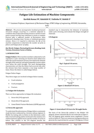
1. International Research Journal of Engineering and Technology (IRJET) e-ISSN: 2395-0056
Volume: 05 Issue: 06 | June-2018 www.irjet.net p-ISSN: 2395-0072
© 2018, IRJET | Impact Factor value: 6.171 | ISO 9001:2008 Certified Journal | Page 1328
Fatigue Life Estimation of Machine Components
Karthik Kumar M1, Rakshith N2, Yathisha N3, Rohith S4
1,2,3,4 Assistant Professor, Department of Mechanical Engg, ATME College of engineering, MYSURU, Karnataka,
India
---------------------------------------------------------------------***---------------------------------------------------------------------
Abstract - The process of progressive localized permanent
structural changes occurring in a material subjected to
conditions that produce fluctuating stressesorstrainsatsome
point or points and that may culminate in cracks or complete
fracture after a sufficient number of fluctuations when
subjected to Bending, Axial, Torsion or combined equivalent
stresses. Hence it is required to determine the life of the
machine components to determine the number of cycles to
failure and Fatigue factor of safety.
Key Words: Fatigue, Fluctuating Stresses,Bending,Axial,
Torsion, Structural, Factor of Safety.
1. INTRODUCTION
Fatigue Failure: Often machine members subjected to such
repeated or cyclic stressing are found to have failed even
when the actual maximum stresses were below the ultimate
strength of the material, and quitefrequentlyatstressvalues
even below the yield strength. The most distinguishing
characteristics are that the failure had occurred only after
the stresses have been repeated a very large number of
times. Hence the failure is called fatigue failure.
Fatigue Failure Stages
Thus three stages are involved in fatigue failure namely,
 Crack initiation.
 Crack propagation.
 Fracture.
1.1 Fatigue life Evaluation
There are three approaches to fatigue life evaluation:
1. Stress-life (S-N) approach.
2. Strain-life (ℰ-N) approach.
3. LinearElastic FractureMechanics(LEFM)approach.
1.2 Stress life approach
To understand the phenomena offatiguefailurea systematic
study has been conducted by a German railway engineer A.
Wohler by testing axles to failure in the laboratory under
fully reversed loading and his work lead to the existenceofa
relation between applied stress and the number of cycles to
failure. This relation or the S-N diagram became the
standard way to characterize the behavior of materials
under cyclic stressing, and evaluate the fatigue strength of
materials.
S-N diagram
Fig 1: Typical S-N curves.
Figure 2: Idealized S-N Curve.
Figure 3: Generalized S-N Curve for Wrought Steels.
The basis of the Stress-Life method is the Wohler S-N
diagram, shown schematically for two materials in Figure 1.
The S-N diagram plots nominal stress amplitude S versus
cycles to failureN. There are numerous testingproceduresto
generatethe required data for a proper S-N diagram.S-Ntest

2. International Research Journal of Engineering and Technology (IRJET) e-ISSN: 2395-0056
Volume: 05 Issue: 06 | June-2018 www.irjet.net p-ISSN: 2395-0072
© 2018, IRJET | Impact Factor value: 6.171 | ISO 9001:2008 Certified Journal | Page 1329
data are usually displayed on a log-log plot, with the actual S-
N line representing the mean of the data from several tests.
S-N curves obtained under torsion or bending load control
test conditions often do not have data at the shorter fatigue
lives (say less than 103 cycles) due to significant plastic
deformation.
2. Power relationship
When plotted on a log-log scale, an S-N curve can be
approximated by a straight line as shown in Figure 2. A
power law equation can then be used to define the S-N
relationship:
Snf = A (Nf) b (1)
Or Sf = Su (Nf)b (2)
Or Sf = 10c (N)b (3)
Where,
C = Log10 and
b = Log10 (4)
b is the slope of the line sometimes referred to as the
Basquin slope.
Given the Basquin slope and any coordinate pair (N, S) on
the S-N curve, the power law equation calculates the cycles
to failure for a known stress amplitude and is given by,
N = (5)
The power relationship is only valid for fatigue lives thatare
on the design line. For ferrous metals this range is from 103
to 106cycles. For non-ferrous metals, this range is from
1x103 to 5x108 cycles.
Fatigue Ratio (Relating Fatigue to Tensile Properties)
The ratio of the endurance limit Se to the ultimate strength
Su of a material is called the fatigue ratio. It has values that
range from 0.25 to 0.60, depending on the material.
For steel, the endurance strength can be approximated by:
Steel 0.5Su for Su <1400 Mpa
Steel 700 Mpa for Su >1400 Mpa
In addition to this relationship, for wrought steels the stress
level corresponding to 1000
Cycles, S1000, can be approximated by:
S1000, Steel = 0.9Su (6)
Utilizing these approximations, a generalized S-N curve for
wrought steels can be created by connectingthe S1000point
with the endurance limit, as shown in Figure 3.
3. Mean Stress and Alternating Stress
Figure 4: Typical Cyclic Loading Parameters..
Cyclical loading can be thought of as a fully reversed
alternating stress superimposed on a constant mean stress
level as shown in figure 3.4. The mean stress is the
arithmetic mean of the maximum stress and the minimum
stress. The alternating stress, also known as the stress
amplitude is then the difference between the peak stresses
and the mean stress. The equations for calculating the mean
stress and alternating stress are as follows:
ϭMean = (7)
ϭalternating = (8)
4. Haigh diagram
Figure 5: Haigh diagram.
The results of a fatigue test using a nonzero mean stress are
often presented in a Haigh diagram, shown in Figure 3.5. A
Haigh diagram plots the mean stress, usually tensile, along
the x-axis and the oscillatory stress amplitude along the y-
axis. Lines of constant life are drawnthroughthedata points.
If the applied stress level is below the endurance limit, the
component is said to have infinite life. If the applied stress
level is above the endurance limit, the component is said to
have finite life. The infinite life region is the regionunderthe
curve and the finite life region is the region above the curve.
For finite life calculations the endurance limit in any of the
models can be replaced with a fully reversed (R = -1)
alternating stress level corresponding to the finite life value
i.e. Snf can be replaced to Sf.

3. International Research Journal of Engineering and Technology (IRJET) e-ISSN: 2395-0056
Volume: 05 Issue: 06 | June-2018 www.irjet.net p-ISSN: 2395-0072
© 2018, IRJET | Impact Factor value: 6.171 | ISO 9001:2008 Certified Journal | Page 1330
A very substantial amount of testing is required to generate
a Haigh diagram, and it is usually impractical to develop
curves for all combinations of meanandalternatingstresses.
Several empirical relationships that relate alternatingstress
to mean stress have been developed to address this
difficulty. These methods define various curves to connect
the endurance limit on the alternating stress axis to either
the yield strength, Sy, ultimate strength Su, or true fracture
stress Sf on the mean stress axis. The following relations are
available in the Stress-Life module:
Goodman (England, 1899) : (9)
Gerber (Germany, 1874) : (10)
Soderberg (USA, 1930) : (11)
Morrow (USA, 1960s) : (12)
Figure 6: Comparison of Mean Stress Equations.
A graphical comparison of these equations is shown in
Figure 6. The Goodman equation was the first attempt at
coming up with a relationship between fatigue and material
properties, using the tensile strength. This wasfollowed bya
slightly more accurateGerberequation,alsousingthetensile
strength, and the slightly less accurate Soderberg equation,
using the yield strength. The Morrow equation improvesthe
accuracy more by using the true fracture stress instead of
the tensile strength. The two most widely accepted methods
are those of Goodman and Gerber. Experience has shown
that test data tends to fall between the Goodman and Gerber
curves. Goodman is often used due to mathematical
simplicity and slightly conservative values.
5. Constant fatigue life diagram
Figure 7: Fatigue and yielding criteria for constant life of
unnotched parts.
Constant fatigue life diagrams relating Sa and Sm are often
modelled is as shown schematically in figure 7. In fig 7, the
intercepts, Sf, at Sm = 0 for a given line found from the fully
reversed, R = -1, modelled S-N curves. In Fatiguedesign with
constant amplitude loading and unnotched parts, if the
coordinates of the applied alternating and meanstressesfall
within the Modified Goodman and Marrow lines shown in
the figure 7, then fatigue failure should not occur priortothe
given life. Note that the difference between the Modified
Goodman and Marrow equations is often rather small; thus
either model often provides similar results. If yielding is not
to occur, then the applied alternating and mean stresses
must fall within the two yield lines connecting ±Sy. If both
fatigue failure and yielding are not to occur, then neither
criterion, as indicated by the three bold lines in the figure 7,
should be exceeded.
6. Modified Goodman Diagram
Figure 8: Modified Goodman chart.
The Modified Goodman diagram shown in Figure .8, account
for yielding as a failure mode. With alternating stress on the
y axis and mean stress on the x axis, we draw a straight line
from the positive fatigue strength to the coordinate
equivalent to the tensile strength on both axes. The
Goodman equation is given as,

4. International Research Journal of Engineering and Technology (IRJET) e-ISSN: 2395-0056
Volume: 05 Issue: 06 | June-2018 www.irjet.net p-ISSN: 2395-0072
© 2018, IRJET | Impact Factor value: 6.171 | ISO 9001:2008 Certified Journal | Page 1331
7. Procedure to find the life of the component
1) If the component is circular get the diameter of the
component.
2) Calculate either of the below from preliminary
calculations.
i) Torsional moment (Tmax &Tmin, N-mm).
ii) Bending moment (Mmax &Mmin, N-mm).
iii) Axial force (Fmax &Fmin, N).
3) Calculate the stresses:
(a)Torsional Stress: Tmax = (13)
Tmin = (14)
(b) Bending Stress: Mmax = (15)
Mmin = (16)
(c) Axial Stress: Fmax = (17)
Fmin = (18)
4) Calculate the alternating stress and mean stress:
(a) Torsion: Ta = (19)
Tm = (20)
(b) Bending: Ma = (21)
Mm = (22)
(c) Axial: Sa = (23)
Sm = (24)
5) Calculate the equivalent stress for the following
combined loading
(a) For Bending and Axial:
Alternating stress (Bending + Axial)
S = Ma+Sa (25)
Mean stress (Bending + Axial)
S = Ma+Sa (26)
Principal stress S1, 2 = (27)
Calculate the principle stresses S1, 2 and find equivalent
stress. By von-mises stress equation
Seq alt = (28)
Seq Mean = (29)
Now calculate Smax and Smin by
Smax = SeqMean + Seqalt (30)
Smin = Seq Mean - Seqalt (31)
(b) For Bending and Torsion:
Find the equivalent stress by using,
Meq max = (32)
Teq max = (33)
Meqmin (34)
Teq min = (35)
From von-mises stress equation,
SMax = (36)
SMin = (37)
6) From Goodman equation we have,
(38)
7) Calculate fully reversed fatigue limit Sf:
Sf = (39)
8) Find the number of cycles to failure[6]:
By power relationship we have,
Sf = 10c (N)b
Where,
C = Log10 (40)
b = Log10 (41)
N = * (42)
8. Procedural steps followedtofindthenumberofcycles
to failure
1. The component is circular and the diameter of the
component is,
Diameter = 30 mm.
2. Calculate either of the below from preliminary
calculations:
i. Torsional moment
Tmax = 1590500 N-mm
Tmin = 530143 N-mm
ii. Bending moment
Mmax = 530143 N-mm
Mmin = 397607 N-mm
iii. Axial force

5. International Research Journal of Engineering and Technology (IRJET) e-ISSN: 2395-0056
Volume: 05 Issue: 06 | June-2018 www.irjet.net p-ISSN: 2395-0072
© 2018, IRJET | Impact Factor value: 6.171 | ISO 9001:2008 Certified Journal | Page 1332
Fmax = 282743 N
Fmin = 353429 N
3. Calculate the stresses:
i. Torsional Stress:
From equation (13) & (14)
Tmax = 300 Mpa
Tmin = 100 Mpa
ii. Bending Stress:
From equation (15) & (16)
Mmax = 200 Mpa
Mmin = 150 Mpa
iii. Axial Stress:
From equation (17) & (18)
Smax = 400 Mpa
Smin = 500 Mpa
4. Calculate the alternating stress and mean stresses:
i. Torsion:
From equation (19) & (20)
Ta = 100 Mpa
Tm = 200 Mpa
ii. Bending:
From equation (20) & (21)
Ma = 25 Mpa
Mm = 175 Mpa
iii. Axial:
From equation (21) & (22)
Sa = -50 Mpa
Sm = 450 Mpa
5. Calculate the equivalent stress for the following
combined loading
i. For bending and axial:
From equation (25)
Alternating stress (Bending + Axial)
Sa = -25 Mpa
From equation (26)
Mean stress (Bending + Axial)
Sm = 625 Mpa
From equation (27)
Principal stress
Sa1 = 88.27 Mpa
Sa2 = -113.2 Mpa
Sm1 = 683.5 Mpa
Sm2 = -58.52 Mpa
By von-mises stress equation (28) & (29)
Seq alt = 174.9 Mpa
Seq Mean = 714.4 Mpa
Now calculate Smax and Smin from equation
(30) & (31)
Smax = 889.4 Mpa
Smin = 539.5 Mpa
ii. For bending and torsion:
From equation (32)
Meq max = Mpa
From equation (33)
Teq max = 360.5 Mpa
From equation (34)
Meq min = 165.13 Mpa
From equation (35)
Teq min = Mpa
From von-mises stress equation, (36) & (37)
SMax = Mpa
SMin = Mpa
6. Get the following inputs from any of the above
calculations to find the number of cycles to failure
for example consider the given data below.
i. Maximum Stress
Smax = 300 Mpa
ii. Minimum stress
Smin = 100 Mpa
iii. Ultimate strength
Su = 690 Mpa
iv. Yield strength
Sy = 580 Mpa
v. Endurance strength
Se = 175.6 Mpa
From equation (23) & (24)
Sa = 100 Mpa
Sm = 200 Mpa
7. Calculate fully reversed fatigue limit Sf from
equation (39)
Sf = 140.81 Mpa
8. Find the number of cycles to failure from equation
(42):
From equation (40) & (41)
c = 3.341
b = -0.1828
Therefore number of cycles to failurefromequation
(42)
N = 3.33*106 cycles
9. Results and Discussions

6. International Research Journal of Engineering and Technology (IRJET) e-ISSN: 2395-0056
Volume: 05 Issue: 06 | June-2018 www.irjet.net p-ISSN: 2395-0072
© 2018, IRJET | Impact Factor value: 6.171 | ISO 9001:2008 Certified Journal | Page 1333
The material used may be either steel, cast iron, cast steel,
wrought aluminium alloy or cast aluminium alloy and the
surface finish of the material may be either Ground,
Machined /cold drawn, hot rolled or As-forged. The
component used is subjected to Bending, Axial or Torsional
loads. The maximum and minimum working stress is found
by preliminary calculation or stressanalysis.Fromtheabove
inputs the following details can be obtained,
1. The Number of cycles to failure, N in cycles.
2. If the working stress falls below the Modified
Goodman line, the componentissaidtohaveinfinite
number of cycles.
3. If the working stress falls above the Modified
Goodman line, the component is said to have finite
number of cycles.
Finally from the above calculation we can conclude that the
number of cycles to failure for the steel componentisinfinite
and the fatigue factor of safety n, required is 1.16.
REFERENCES
[1] Joseph E. Shigley’s, Standard handbook of Machine
design.
[2] Shigley’s, Mechanical engineering design.
[3] R.S Kurmi, J.K Guptha, Machine design.
[4] Ralph I. Stephens, Ali.Fatemi, Robert R. Stephens, Henry
O. Fuchs, Metal fatigue in engineering.
[5] Julie A. Bannantine, Jess J. Comer, James L. Handrock,
Fundamentals of Metal fatigue analysis.